IBL, or image-based lighting, is a set of technologies for illuminating objects, not by directly analyzing light as in the previous chapter, but by treating the surrounding environment as a large light source. This is usually done by manipulating a cube map environment map (taken from the real world or generated from a 3D scene) so that we can use it directly in our lighting equation: treat each cube texture element as a light emitter light emitter. In this way, we can effectively capture the global light and overall sense of the environment, so that objects have a better sense of belonging in their environment.

Because image-based lighting algorithms capture lighting for certain (global) environments, their inputs are considered to be more accurate forms of ambient lighting, or even a rough approximation of global lighting. This makes IBL interesting for PBR s because objects seem more physically accurate when we consider the lighting of the environment.

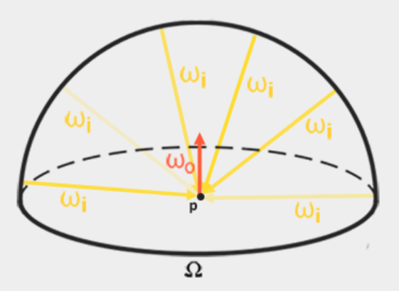
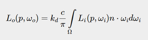
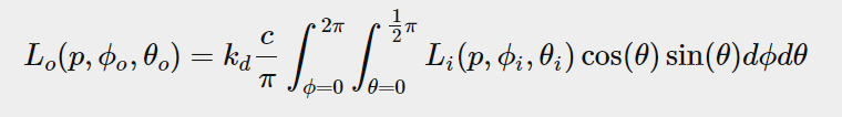
To begin introducing IBL into our PBR system, let's take a quick look at the reflectance equation again:

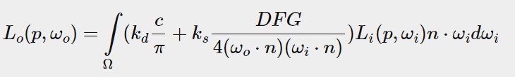
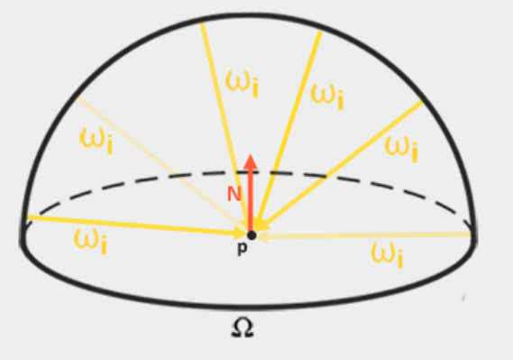
As mentioned earlier, our main objective is to solve the integrals of all incoming light directions wi on a hemispherical omega. It is easy to solve the integral in the previous chapter because we know in advance the exact light direction wi that contributes to the integral. However, this time, each incoming light direction wi from the surrounding environment may have some radiation, which makes solving the integral much easier. This gives us two main requirements for solving integrals:

1. Given any direction vector wi, we need some methods to retrieve the radiosity of the scene.
2. Solving integrals needs to be fast and real-time.
Now, the first requirement is relatively easy. We've already implied that, but one way to represent environmental or scene irradiance is in the form of (processed) environmental cube maps. Given such a cube map, we can visualize each ridge element of the cube map as a single emitting light source. By sampling this cube map with any direction vector wi, we retrieve the radiosity of the scene from that direction.

Given any direction vector wi, it is very simple to obtain the radiance of a scene:

//Obtaining the color of cubemap from an angle
vec3 radiance = texture(_cubemapEnvironment, w_i).rgb;  

Nevertheless, solving the integral requires that we not only sample the environment map from one direction, but also from all possible directions wi on the hemisphere ome omega, which is too expensive for each fragment shader call. In order to solve the integral in a more efficient way, we need to preprocess or pre-compute most of the calculations. For this reason, we must study the reflection equation more deeply:

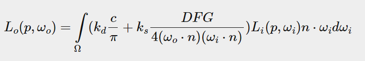
Looking at the reflection equation carefully, we find that the diffuse kd and mirror ks terms of BRDF are independent of each other, and we can divide the integral into two parts:

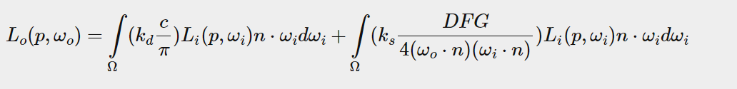
By dividing the integral into two parts, we can focus on the diffuse and mirror reflections, respectively. The focus of this chapter is on the diffusion integral.

Looking closely at the diffusion integral, we find that the diffuse lambert term diffuse Lambert term is a constant term (color c, refractive index kd, and PI are constant on the integral) and independent of any integral variable. For this reason, we can move the constant term out of the diffusion integral:

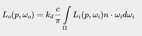
This gives us an integral that only depends on wi (assuming p is at the center of the environment map). With this knowledge, we can calculate or precompute a new cube map, which is stored in each sample direction (or texture pixels), and convolute to obtain the results of the diffuse reflection integral.

Considering all the other entries in the dataset, convolution is applying some calculations to each entry in the dataset. A dataset is a radiometric or environmental map of a scene. Therefore, for each sampling direction in a cube map, all other sampling directions on the hemisphere ome Omega are taken into account.

In order to integral the environment map, we solve the integral of each output wo sampling direction by discretely sampling a large number of directions wi on the hemisphere_and averaging their radiation. The hemisphere in which we construct the sample direction wi faces the output sample direction that we are convoluting.

(Understanding: in the formula, kd,c,pi are all proposed as constants, only the wi integral needs to be calculated, and the wi integral can be expressed directly by a cubemap)

 

This precomputed cube map, which stores the integral results for wo in each sampling direction, can be thought of as the sum of the precomputed indirect diffuse light of all the scenes that shines onto a surface aligned with wo in the direction. Such cube maps are called irradiance map s because convoluted cube maps effectively allow us to directly sample (pre-computed) the irradiance of a scene from any direction.

The radiation equation also depends on position p, which is assumed to be at the center of the radiation map. This does mean that all diffuse indirect light must come from a single environmental map, which may break the illusion of reality (especially indoors). The rendering engine solves this problem by placing reflection probes throughout the scene, each of which calculates its own irradiance map of the surrounding environment. Thus, the irradiance (and radiance) at position P is the interpolated irradiance between its nearest reflector probe. Now let's assume that we always sample the environment map from the center.

Below is a cube map environment map and the resulting irradiance map (from wave engine The wave engine provides) an example, averaging the radiance of the scene for wo in each direction.

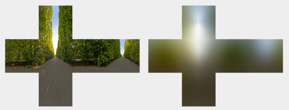
By storing the convoluted convolution results in each cube map texture pixel (in the direction of wo), the display of the irradiance map is somewhat like the average color or illumination display of the environment. Sampling from any direction in this environmental map will give us the illumination of the scene in that particular direction. (

1.PBR and HDR (Physic Based Render   and  High Dynamic Range)

We outlined it in the previous chapter: It is important to consider the high dynamic range of scene lighting in PBR pipes. Since most of the input to PBR is based on real physical properties and measurements, it is meaningful to closely match the incoming light values to their physical equivalents. Whether we make a valid guess about the radiation flux of each lamp or use their direct physical equivalent, the difference between a simple bulb or the sun is significant. It is not possible to correctly specify the relative intensity of each light without working in an HDR rendering environment.

So PBR and HDR go hand in hand, but how do they relate to image-based lighting? As we have seen in the previous chapter, it is relatively easy for PBR to work in HDR. However, for image-based lighting, we base the indirect light intensity of the environment on the color value of the environment cube map, and we need some way to store the high dynamic range of lighting in the environment map.

So far, we have been using environment maps as cube maps (for example, as sky boxes) in low dynamic range (LDR). We use them directly to derive color values from personal facial images, ranging from 0.0 to 1.0, and process them as they are. Although this may be good for visual output, it does not work when they are used as physical input parameters.

1.1 The radiance HDR file format (Radiation HDR file format)

Enter The radiance HDR file format radiation file format. The radiance file format (extension.hdr) stores a complete cube map with all six faces as floating-point data. This allows us to specify color values that range from 0.0 to 1.0 to give the light the correct color intensity. The file format also uses a clever trick to store each floating-point value, not 32 bits per channel, but 8 bits per channel, using the alpha channel of color as an index (which really loses accuracy). This works well, but the parser needs to convert each color back to its equivalent floating point number.

There are many radiometric HDR environment maps available from sIBL archive Free from other sources, you can see an example below:

 

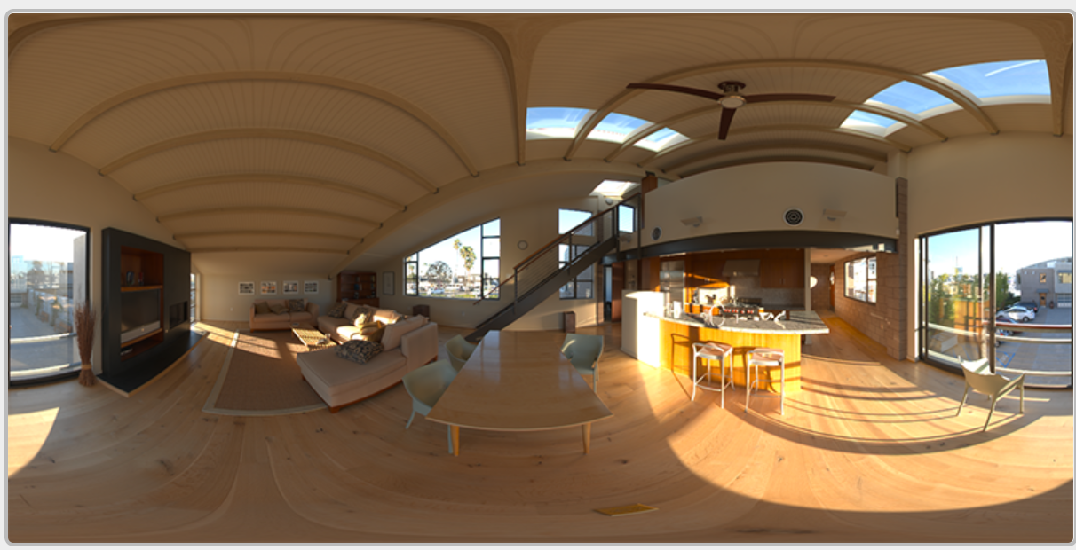
This may not be what you expected, because the image looks distorted and does not display any of the six separate cube patches of the environment map we saw earlier. This environment map is projected from a sphere onto a plane so that we can more easily store the environment in a single image, called an equirectangular map. This does have a small warning because most of the visual resolution is stored in the horizontal view direction and less is preserved at the bottom and top. In most cases, this is a good compromise because almost all renderers will find most of the interesting lighting and environment in the horizontal viewing direction.

 

1.2 HDR and stb_image.h

Loading radiance HDR images directly requires some knowledge of file formats, which is not too difficult, but also cumbersome. Fortunately, the popular headstore stb_image.h supports loading radiated HDR images directly into an array of floating point values floating point value arrays, which fully meets our needs. Will stb_ Once an image has been added to your project, loading an HDR image is now very simple, as shown below:

#include "stb_image.h"
[...]

stbi_set_flip_vertically_on_load(true);
int width, height, nrComponents;
float *data = stbi_loadf("newport_loft.hdr", &width, &height, &nrComponents, 0);
unsigned int hdrTexture;
if (data)
{
    glGenTextures(1, &hdrTexture);
    glBindTexture(GL_TEXTURE_2D, hdrTexture);
    glTexImage2D(GL_TEXTURE_2D, 0, GL_RGB16F, width, height, 0, GL_RGB, GL_FLOAT, data); 

    glTexParameteri(GL_TEXTURE_2D, GL_TEXTURE_WRAP_S, GL_CLAMP_TO_EDGE);
    glTexParameteri(GL_TEXTURE_2D, GL_TEXTURE_WRAP_T, GL_CLAMP_TO_EDGE);
    glTexParameteri(GL_TEXTURE_2D, GL_TEXTURE_MIN_FILTER, GL_LINEAR);
    glTexParameteri(GL_TEXTURE_2D, GL_TEXTURE_MAG_FILTER, GL_LINEAR);

    stbi_image_free(data);
}
else
{
    std::cout << "Failed to load HDR image." << std::endl;
}  

stb_image.h Automatically maps HDR values to a list of floating-point values: by default, 32 bits per channel and 3 channels per color. That's all we need to store equirectangular HDR environment maps in 2D floating-point textures.

1.3 From Equirectangular to Cubemap (from Equirectangular to Cubemap)

You can use equirectangular maps directly for environment lookups, but these operations can be relatively expensive, in which case direct cubemap sample cube mapping sampling has higher performance. Therefore, in this chapter, we will first convert the equirectangular image to a cube map for further processing. Note that during this process, we also show you how to sample the equirectangular map as if it were a 3D environment map, in which case you are free to choose any solution you like.

To convert an equirectangular image to a cube map, we need to render a (unit) cube and project the equirectangular map from the inside onto all faces of the cube, and take six images for each side of the cube as the cube map surface. The vertex shader of this cube simply renders the cube and passes its local location as a 3D sample vector to the fragment shader fragment shader:

#version 330 core
layout (location = 0) in vec3 aPos;

out vec3 localPos;

uniform mat4 projection;
uniform mat4 view;

void main()
{
    localPos = aPos;  
    gl_Position =  projection * view * vec4(localPos, 1.0);
}

For the Fragment Shader, we color each part of the cube as if we were collapsing the equirectangular map neatly to each side of the cube. To achieve this, we interpolate the sample direction of the fragment as interpolated from the local position of the cube, then sample it using this direction vector and some triangular magic (spherical to cartesian sphere to Cartesian cartesian) equivalent rectangular maps as if it were a cube map itself. We store the results directly in the cube fragments, which should be all we need to do:

#version 330 core
out vec4 FragColor;
in vec3 localPos;

uniform sampler2D equirectangularMap;

const vec2 invAtan = vec2(0.1591, 0.3183);

//Sample spherical surfaces, convert uv using mathematical formulas
vec2 SampleSphericalMap(vec3 v)
{
    vec2 uv = vec2(atan(v.z, v.x), asin(v.y));
    uv *= invAtan;
    uv += 0.5;
    return uv;
}

void main()
{		
    //Sampling spherical surface
    vec2 uv = SampleSphericalMap(normalize(localPos)); // make sure to normalize localPos
    vec3 color = texture(equirectangularMap, uv).rgb;
    
    FragColor = vec4(color, 1.0);
}

If you render a cube in the center of the scene given an HDR equirectangular map, you will get something like this:

This indicates that we are effectively mapping equirectangular images to cubes, but it does not help us convert source HDR images to cube-mapped textures. To achieve this, we must render the same cube six times, view each side of the cube, and record its visual results using the Frame Buffer object:

Configure framebuffer:

unsigned int captureFBO, captureRBO;
glGenFramebuffers(1, &captureFBO);
glGenRenderbuffers(1, &captureRBO);

glBindFramebuffer(GL_FRAMEBUFFER, captureFBO);
glBindRenderbuffer(GL_RENDERBUFFER, captureRBO);
glRenderbufferStorage(GL_RENDERBUFFER, GL_DEPTH_COMPONENT24, 512, 512);
glFramebufferRenderbuffer(GL_FRAMEBUFFER, GL_DEPTH_ATTACHMENT, GL_RENDERBUFFER, captureRBO); 

Of course, we will then generate the corresponding cube map color texture, which pre-allocates memory for each of its six faces:

//Initialize cubemap
unsigned int envCubemap;
glGenTextures(1, &envCubemap);
glBindTexture(GL_TEXTURE_CUBE_MAP, envCubemap);
//Configure each face
for (unsigned int i = 0; i < 6; ++i)
{
    // note that we store each face with 16 bit floating point values
    // Declare that each face is a floating point number
    glTexImage2D(GL_TEXTURE_CUBE_MAP_POSITIVE_X + i, 0, GL_RGB16F, 
                 512, 512, 0, GL_RGB, GL_FLOAT, nullptr);
}
glTexParameteri(GL_TEXTURE_CUBE_MAP, GL_TEXTURE_WRAP_S, GL_CLAMP_TO_EDGE);
glTexParameteri(GL_TEXTURE_CUBE_MAP, GL_TEXTURE_WRAP_T, GL_CLAMP_TO_EDGE);
glTexParameteri(GL_TEXTURE_CUBE_MAP, GL_TEXTURE_WRAP_R, GL_CLAMP_TO_EDGE);
glTexParameteri(GL_TEXTURE_CUBE_MAP, GL_TEXTURE_MIN_FILTER, GL_LINEAR);
glTexParameteri(GL_TEXTURE_CUBE_MAP, GL_TEXTURE_MAG_FILTER, GL_LINEAR);

Then all that remains is to capture the equirectangular 2D texture onto the cube surface.

Like before framebuffer Frame buffer and point shadows The code details discussed in the Point Shadow section come down to six different view matrices (facing each side of the cube), a projection matrix with a 90-degree fov view to capture the entire face, render a cube six times, and store the results in a floating-point frame buffer:

//Configure 6 views toward fov matrix
glm::mat4 captureProjection = glm::perspective(glm::radians(90.0f), 1.0f, 0.1f, 10.0f);
glm::mat4 captureViews[] = 
{
   glm::lookAt(glm::vec3(0.0f, 0.0f, 0.0f), glm::vec3( 1.0f,  0.0f,  0.0f), glm::vec3(0.0f, -1.0f,  0.0f)),
   glm::lookAt(glm::vec3(0.0f, 0.0f, 0.0f), glm::vec3(-1.0f,  0.0f,  0.0f), glm::vec3(0.0f, -1.0f,  0.0f)),
   glm::lookAt(glm::vec3(0.0f, 0.0f, 0.0f), glm::vec3( 0.0f,  1.0f,  0.0f), glm::vec3(0.0f,  0.0f,  1.0f)),
   glm::lookAt(glm::vec3(0.0f, 0.0f, 0.0f), glm::vec3( 0.0f, -1.0f,  0.0f), glm::vec3(0.0f,  0.0f, -1.0f)),
   glm::lookAt(glm::vec3(0.0f, 0.0f, 0.0f), glm::vec3( 0.0f,  0.0f,  1.0f), glm::vec3(0.0f, -1.0f,  0.0f)),
   glm::lookAt(glm::vec3(0.0f, 0.0f, 0.0f), glm::vec3( 0.0f,  0.0f, -1.0f), glm::vec3(0.0f, -1.0f,  0.0f))
};

// convert HDR equirectangular environment map to cubemap equivalent
// Initialize rendering of spherical environment map
equirectangularToCubemapShader.use();
equirectangularToCubemapShader.setInt("equirectangularMap", 0);
equirectangularToCubemapShader.setMat4("projection", captureProjection);
glActiveTexture(GL_TEXTURE0);
glBindTexture(GL_TEXTURE_2D, hdrTexture);

glViewport(0, 0, 512, 512); // don't forget to configure the viewport to the capture dimensions.
glBindFramebuffer(GL_FRAMEBUFFER, captureFBO);
//Render six faces of cubemap from six perspectives
for (unsigned int i = 0; i < 6; ++i)
{
    equirectangularToCubemapShader.setMat4("view", captureViews[i]);
    glFramebufferTexture2D(GL_FRAMEBUFFER, GL_COLOR_ATTACHMENT0, 
                           GL_TEXTURE_CUBE_MAP_POSITIVE_X + i, envCubemap, 0);
    glClear(GL_COLOR_BUFFER_BIT | GL_DEPTH_BUFFER_BIT);

    renderCube(); // renders a 1x1 cube
}
glBindFramebuffer(GL_FRAMEBUFFER, 0);  

We take the color attachment of the frame buffer and switch the texture target for each face of the cube map, rendering the scene directly into one face of the cube map. Once this routine is complete (we only need to do it once), the cube map envCubemap should be the cube map environment version of our original HDR image.

Let's show the cube map around us by writing a very simple sky box shader to test the cube map:

#version 330 core
layout (location = 0) in vec3 aPos;

uniform mat4 projection;
uniform mat4 view;

out vec3 localPos;

void main()
{
    localPos = aPos;

    mat4 rotView = mat4(mat3(view)); // remove translation from the view matrix
    vec4 clipPos = projection * rotView * vec4(localPos, 1.0);

    gl_Position = clipPos.xyww;
}

Note the xyww technique here, which ensures that the depth value of the rendered cube fragment always ends at 1.0, the maximum depth value, as described in the Cube Mapping chapter. Note that we need to change the depth comparison function to GL_LEQUAL:

glDepthFunc(GL_LEQUAL);  

(These are the two steps that the cubemap environment map must configure)

The segment shader then uses the local segment location of the cube to directly sample the cube map environment map:

#version 330 core
out vec4 FragColor;

in vec3 localPos;
  
uniform samplerCube environmentMap;
  
void main()
{
    vec3 envColor = texture(environmentMap, localPos).rgb;
    // hdr
    envColor = envColor / (envColor + vec3(1.0));
    // gamma correction
    envColor = pow(envColor, vec3(1.0/2.2)); 
  
    FragColor = vec4(envColor, 1.0);
}

The environment map is sampled using an interpolation vertex cube location that directly corresponds to the correct sampling direction vector. Rendering the shader on the cube should give you a map of the environment as a background that does not move when you see that the camera's panning component is ignored. In addition, since we output the HDR values of the environment map directly to the default LDR frame buffer, we want the color values to be tone map the color values hue mapped correctly. In addition, almost all HDR maps are in linear color space by default, so we need to apply gamma correction before writing to the default frame buffer.

Now rendering the sampled environment map on the previously rendered sphere should look like this:

Hmm... We spent a lot of settings getting here, but we successfully read the HDR environment map, converted it from an equidistant rectangle map to a cube map, and rendered the HDR cube map into the scene as a sky box. In addition, we have set up a small system to render all six faces of the cube map, which we will need again when convoluting the environment map.

2. Cubemap convolution

As mentioned at the beginning of this chapter, our main goal is to solve the integral for all diffuse indirect lighting given the scene's irradiance in the form of a cubemap environment map to solve all diffuse indirect lighting integral s for a given scene irradiance in the form of a cubemap environment map. We know that we can obtain the radiosity of scene L(p,wi) in a particular direction by sampling the HDR environment map on the direction wi. To solve the integral problem, we must sample each segment from all possible directions of the scene radiation within the hemisphere ome omega.

However, it is not computationally possible to sample light from the environment in every possible direction (in omega), and the number of possible directions is theoretically infinite. However, we can approximate the number of directions by taking a finite number of directions or samples, spaced uniformly or taken randomly from within the hemisphere, to get a fairly accurate approximation of the irradiance; effectively solving the integral discretely approximates the number of directions by uniformly or randomly sampling a limited number of directions or samples from the hemisphere to obtain a fairly accurate approximation of the irradiance; Solving integrals effectively and discretely

However, it is still too expensive to do this for each fragment in real time because the number of samples required is very large to achieve good results, so we want to precompute. Since the direction of the hemisphere determines where we capture the irradiance, we can pre-calculate the irradiance for every possible hemisphere orientation around all outgoing directions Wo to pre-calculate the irradiance in each possible hemisphere direction around all outgoing directions wo:

Given any direction vector wi in the illumination channel, we can then sample the pre-computed illumination map to retrieve the total diffuse illumination from the direction wi. To determine the amount of indirectly diffused (irradiated) light on a fragment surface, we retrieve the total irradiance of the hemisphere oriented around its surface normal. It's easy to get the irradiance of a scene:

vec3 irradiance = texture(irradianceMap, N).rgb;

Now, to generate an irradiance map, we need to convert the light from the environment into a cube map. Assuming that for each segment, the hemisphere of the surface is oriented along the normal vector N, the convoluting a cubemap convolution cube map is equal to calculating the total average radiance of wi in each direction in the N-oriented hemisphere_.

Fortunately, all the tedious settings in this chapter are not futile, because we can now get the converted cube map directly, convolute it in the segment shader, and use the frame buffers rendered to all six faces to capture its results in the direction of the new cube map. Since we've set it to convert equirectangular environment maps to cube maps, we can use the exact same method, but with different fragment shaders:

#version 330 core
out vec4 FragColor;
in vec3 localPos;

uniform samplerCube environmentMap;

const float PI = 3.14159265359;

void main()
{		
    // Sampling direction is equivalent to hemispherical direction
    // the sample direction equals the hemisphere's orientation 
    vec3 normal = normalize(localPos);
  
    vec3 irradiance = vec3(0.0);
  
    [...] // convolution code
  
    FragColor = vec4(irradiance, 1.0);
}

Environment Map is a HDR cube map converted from equirectangular HDR environment map.

There are many ways to convolute an environmental map, but in this chapter, we will generate a fixed number of sample vectors for each cube map texture pixel, surround the sample direction along the hemisphere_direction, and average the results. A fixed number of sample vectors will be evenly distributed in the hemisphere. Note that the integral is a continuous function and that discrete sampling of its function will be an approximation given a fixed number of sample vectors. The more sample vectors we use, the closer we get to the integral.

The integral of the reflection equation rotates around the stereo angle dw, which is difficult to handle. We are not integrating on the stereo angle dw, but in its equivalent spherical coordinates θ and φ Upper integral.

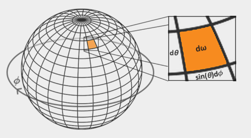
We use the polar azimuth ϕ angle to sample around the ring of the hemisphere between 0 and 2 pi, and use the inclination zenith θ angle between 0 and 0.5 pi to sample the increasing rings of the hemisphere( φ Horizontal rotation angle, θ Is the upward angle)

(where cos θ = N * COS in wi θ, and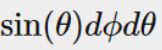Is the area of dwi)

Solving the integral requires us to collect a fixed number of discrete samples within a hemisphere of Omega and average their results. This converts the integral into the following discrete versions based on the n1 and n2 discrete samples given in each spherical coordinate Riemann sum Riemann and: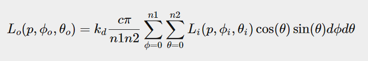

When we sample two spherical values discretely, each sample approximates or averages an area on the hemisphere, as shown in the previous image. Note (due to the general nature of the sphere) that the zenith angle occurs when the sample area converges to the top of the center θ The higher the hemisphere, the smaller the discrete sample area. To compensate for smaller regions, we press sin θ Scale the area to measure its contribution.

Given the spherical coordinates of the integral, discrete sampling of the hemisphere is converted to the following fragment code:

vec3 irradiance = vec3(0.0);  

vec3 up    = vec3(0.0, 1.0, 0.0);
vec3 right = normalize(cross(up, normal));
up         = normalize(cross(normal, right));

float sampleDelta = 0.025;
float nrSamples = 0.0; 
// Yes φ Integrate
for(float phi = 0.0; phi < 2.0 * PI; phi += sampleDelta)
{
    //Yes θ Integrate
    for(float theta = 0.0; theta < 0.5 * PI; theta += sampleDelta)
    {
        // spherical to cartesian (in tangent space)
        // Spherical coordinate system converted to xyz Cartesian coordinate system, x=sin θ* Cos φ,  y = sin θ* Sin φ,  z=cos θ
        vec3 tangentSample = vec3(sin(theta) * cos(phi),  sin(theta) * sin(phi), cos(theta));
        // tangent space to world
        vec3 sampleVec = tangentSample.x * right + tangentSample.y * up + tangentSample.z * N; 
        // apply a formula
        irradiance += texture(environmentMap, sampleVec).rgb * cos(theta) * sin(theta);
        nrSamples++;
    }
}
irradiance = PI * irradiance * (1.0 / float(nrSamples));

We specify a fixed sampleDelta delta value to traverse the hemisphere; Reducing or increasing sample increments will increase or decrease accuracy, respectively.

In both loops, we convert two spherical coordinates to a 3D Cartesian sample vector, convert the sample from tangent to normal-oriented world space, and use this sample vector to directly sample the HDR environment map. We add each sample result to the irradiance and divide the total number of samples collected to get the average sample irradiance. Note that we scale the sample color values by cos(theta) because the light is weak at a larger angle and sin(theta) is used to interpret smaller sample areas in the higher hemisphere.

All that remains now is to set up the OpenGL rendering code so that we can convolute the envCubemap we captured earlier. First we create the irradiance cube map (again, we only need to do this once before rendering the loop):

unsigned int irradianceMap;
glGenTextures(1, &irradianceMap);
glBindTexture(GL_TEXTURE_CUBE_MAP, irradianceMap);
for (unsigned int i = 0; i < 6; ++i)
{
    glTexImage2D(GL_TEXTURE_CUBE_MAP_POSITIVE_X + i, 0, GL_RGB16F, 32, 32, 0, 
                 GL_RGB, GL_FLOAT, nullptr);
}
glTexParameteri(GL_TEXTURE_CUBE_MAP, GL_TEXTURE_WRAP_S, GL_CLAMP_TO_EDGE);
glTexParameteri(GL_TEXTURE_CUBE_MAP, GL_TEXTURE_WRAP_T, GL_CLAMP_TO_EDGE);
glTexParameteri(GL_TEXTURE_CUBE_MAP, GL_TEXTURE_WRAP_R, GL_CLAMP_TO_EDGE);
glTexParameteri(GL_TEXTURE_CUBE_MAP, GL_TEXTURE_MIN_FILTER, GL_LINEAR);
glTexParameteri(GL_TEXTURE_CUBE_MAP, GL_TEXTURE_MAG_FILTER, GL_LINEAR);

Since the irradiance map averages all the surrounding radiation evenly, it does not have much high-frequency detail, so we can store the map at a low resolution (32x32), allowing linear filtering of OpenGL to do most of the work. Next, we will resize the capture frame buffer to the new resolution:

glBindFramebuffer(GL_FRAMEBUFFER, captureFBO);
glBindRenderbuffer(GL_RENDERBUFFER, captureRBO);
glRenderbufferStorage(GL_RENDERBUFFER, GL_DEPTH_COMPONENT24, 32, 32);  

Using the convolution shader, we render the environment map in a similar way to how we captured the environment cubemap using a convolution shader, we render the environment map in a similar way to capturing the environment cube map:

//Initialize Rendering
irradianceShader.use();
irradianceShader.setInt("environmentMap", 0);
irradianceShader.setMat4("projection", captureProjection);
glActiveTexture(GL_TEXTURE0);
glBindTexture(GL_TEXTURE_CUBE_MAP, envCubemap);

glViewport(0, 0, 32, 32); // don't forget to configure the viewport to the capture dimensions.
glBindFramebuffer(GL_FRAMEBUFFER, captureFBO);
// Rendering six faces of cubemap
for (unsigned int i = 0; i < 6; ++i)
{
    irradianceShader.setMat4("view", captureViews[i]);
    glFramebufferTexture2D(GL_FRAMEBUFFER, GL_COLOR_ATTACHMENT0, 
                           GL_TEXTURE_CUBE_MAP_POSITIVE_X + i, irradianceMap, 0);
    glClear(GL_COLOR_BUFFER_BIT | GL_DEPTH_BUFFER_BIT);

    renderCube();
}
glBindFramebuffer(GL_FRAMEBUFFER, 0);  

Now, after this routine, we should have a pre-computed irradiance map that we can use directly for illumination based on diffuse reflection images. To see if we successfully convoluted the environment map, we replaced the environment map with the irradiance map as the environment sampler for the sky box:

If it looks like a highly blurred version of an environment map, you have successfully convoluted the environment map

3.PBR and indirect irradiance lighting (PBR and indirect irradiance lighting)

The irradiance graph represents the diffuse part of the reflection integral, accumulated by all surrounding indirect light. Since light does not come from a direct light source, but from the surrounding environment, we consider diffuse and mirror-reflective indirect lighting as ambient lighting, replacing the constants we previously set.

First, make sure that the precomputed irradiance map is added as a cube sampler:

uniform samplerCube irradianceMap;

Given an irradiance map that contains all the indirect diffuse reflections of the scene, retrieving the irradiance of the affected fragment is as simple as retrieving a single texture sample for a given surface normal:

// vec3 ambient = vec3(0.03);
vec3 ambient = texture(irradianceMap, N).rgb;

However, since indirect lighting includes both diffuse and mirror reflections (as we see from the split version of the reflection equation), we need to balance the diffuse reflections accordingly. Similar to what we did in the previous chapter, we use the Fresnel Fresnel equation to determine the indirect reflectance of a surface from which we can derive the refraction (or diffuse) ratio:

vec3 kS = fresnelSchlick(max(dot(N, V), 0.0), F0);
vec3 kD = 1.0 - kS;
vec3 irradiance = texture(irradianceMap, N).rgb;
vec3 diffuse    = irradiance * albedo;
vec3 ambient    = (kD * diffuse) * ao; 

As the ambient light comes from all directions within the hemisphere oriented around the normal N, there's no single halfway vector to determine the Fresnel response. To still simulate Fresnel, we calculate the Fresnel from the angle between the normal and view vector. However, earlier we used the micro-surface halfway vector, influenced by the roughness of the surface, as input to the Fresnel equation. As we currently don't take roughness in account, the surface's reflective ratio will always end up relatively high. Indirect light follows the same properties of direct light so we expect rougher surfaces to reflect less strongly on the surface edges. Because of this, the indirect Fresnel reflection strength looks off on rough non-metal surfaces: (without roughness roughness, edges will always be bright and unnatural)

We can alleviate this problem by injecting a roughness term into the Fresnel-Schlick equation, as described by Slei bastien Lagarde:

vec3 fresnelSchlickRoughness(float cosTheta, vec3 F0, float roughness)
{
    return F0 + (max(vec3(1.0 - roughness), F0) - F0) * pow(clamp(1.0 - cosTheta, 0.0, 1.0), 5.0);
}   

By considering the surface roughness when calculating the Fresnel response, the environment code is ultimately:

vec3 kS = fresnelSchlickRoughness(max(dot(N, V), 0.0), F0, roughness); 
vec3 kD = 1.0 - kS;
vec3 irradiance = texture(irradianceMap, N).rgb;
vec3 diffuse    = irradiance * albedo;
vec3 ambient    = (kD * diffuse) * ao; 

As you can see, the actual image-based illumination calculation is very simple, requiring only a cube map texture lookup. Most of the work is to precompute or convolute irradiance maps.

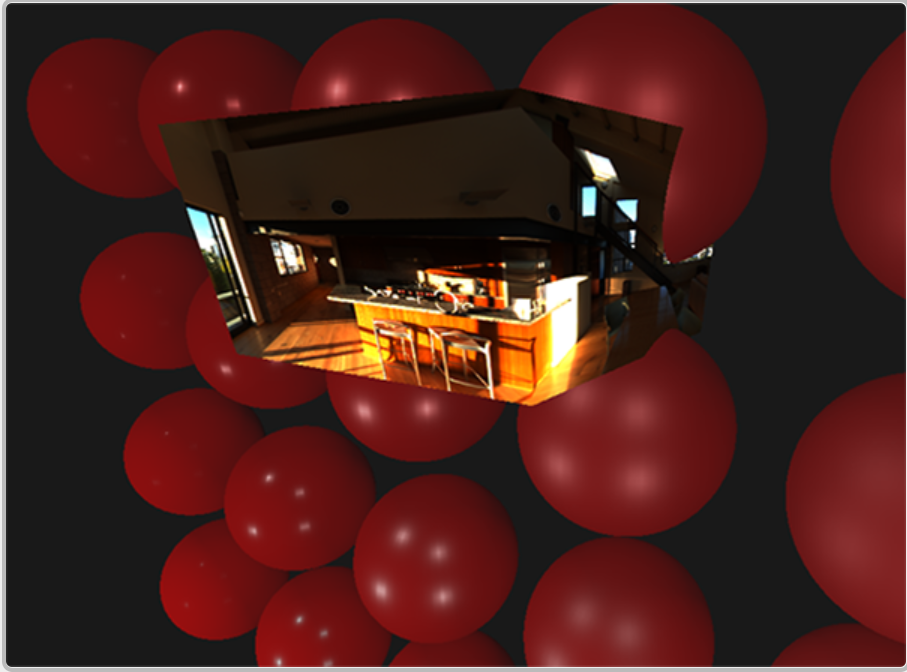
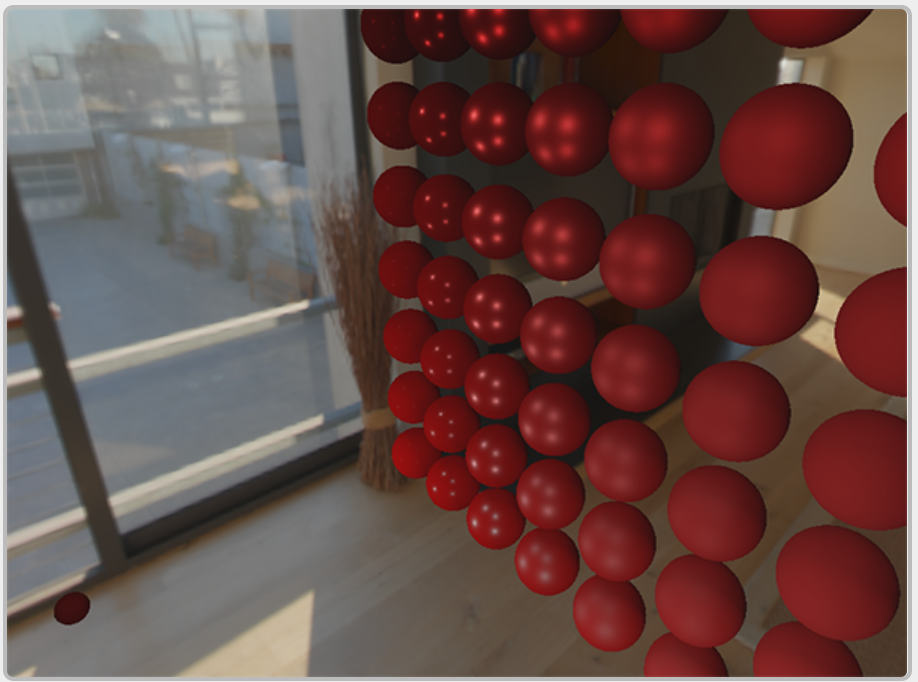
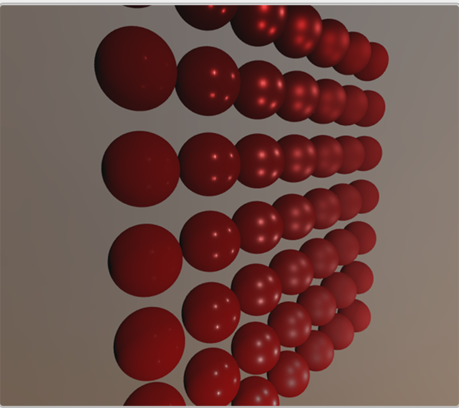
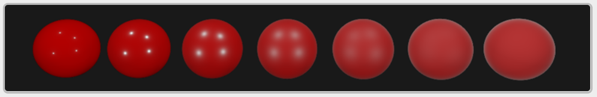
If we take the initial scene from the PBR lighting chapter, where each sphere has a vertically increased metal and a horizontally increased roughness value, and add light based on a diffuse reflection image, it looks a little like this:

​​​​​​​

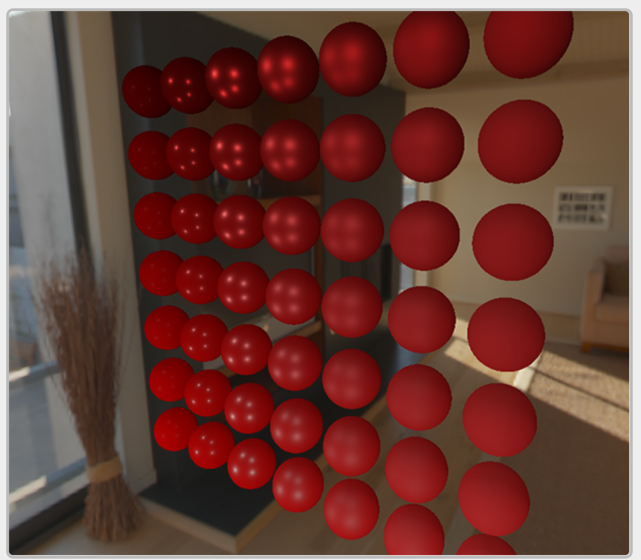
It still looks a bit odd because more metal spheres require some form of reflection to properly start looking like metal surfaces (because they do not reflect diffused light), which currently only (almost) come from point sources. Nevertheless, you can see that spheres do feel more in place in the environment (especially when you switch between environmental maps) because the surface response responds accordingly to the ambient light of the environment.

You can find the full source code for the topic you are discussing here. In the next chapter, we will add the indirect specular reflection part of the reflection integral, at which point we will really see the power of the PBR.