catalogue
(8). Weighted graph and weighted graph
III Implementation of graph structure
(3). The idea of two algorithms
(1). Idea of breadth first search algorithm
(2). Implementation of breadth first search
(1). Idea of depth first search
(2). Implementation of depth first search algorithm
1, Initial graph structure
1. What is a graph
Graph is a kind of data structure similar to tree. In fact, in the mathematical concept, tree is a kind of graph.
Trees can be used to simulate many real data structures, such as genealogy, company organizational structure and so on. At the same time, the subway map can be used to simulate the map:
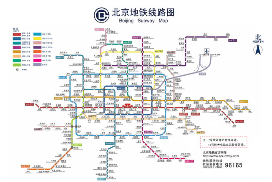
The relationship between the above nodes (actually called vertex vertex in the graph) cannot be represented by a tree (not even a few fork trees). At this time, you can use a graph to simulate them.
2. Features of the drawing
A set of vertices: usually V (Vertex) represents the set of vertices
A set of edges: usually E (Edge) represents the set of edges
An edge is a line between vertices
Edges can be directed or undirected. (for example, A --- B usually means undirected. A -- > b usually means directed)
3. Terminology of Graphs
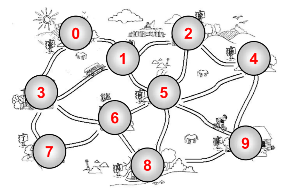
The following figure is an abstract diagram:
(1). vertex
A vertex represents a node in a graph.
For example, a station in a subway station, a village in multiple villages, a host in the Internet, and people in interpersonal relationships.
(2). edge
Edges represent vertices and lines between vertices.
For example, the direct connection between two stations in the subway station is one side.
Note: the edges here are not called paths. Paths have other concepts
In the above figure: 0 - 1 has an edge, 1 - 2 has an edge, 0 - 2 has no edge
(3). Adjacent vertex
Vertices connected by one edge are called adjacent vertices.
For example, 0 - 1 is adjacent and 0 - 3 is adjacent 0 - 2 are not adjacent
(4). degree
The degree of a vertex is the number of adjacent vertices.
For example, vertex 0 is connected with two other vertices, and the degree of vertex 0 is 2
For example, vertex 1 is connected to the other four vertices, and the degree of vertex 1 is 4
(5). route
The path is vertex V1, V2, A continuous sequence of VN, such as 0 1 5 9 in the figure above, is a path
1. Simple path: a simple path requires no duplicate vertices For example, 0 1 5 9 is a simple path
2. Loop: the same path between the first vertex and the last vertex is called a loop For example, 0 1 5 6 3 0
(6). Undirected graph
The graph above is an undirected graph because all edges have no direction.
For example, if there is a change between 0 and 1, it means that this edge can guarantee 0 - > 1 and 1 - > 0
(7). Directed graph
The edges in a directed graph are directional.
For example, 0 - > 1 cannot guarantee 1 - > 0, which should be determined according to the direction
(8). Weighted graph and weighted graph
1. Unauthorized graph
The graph above is a weight free graph (edges do not carry weights)
The edges in our figure above are meaningless. We can't close the 0 - 1 edge, which is farther or longer than the 4 - 9 edge
2. Weighted graph
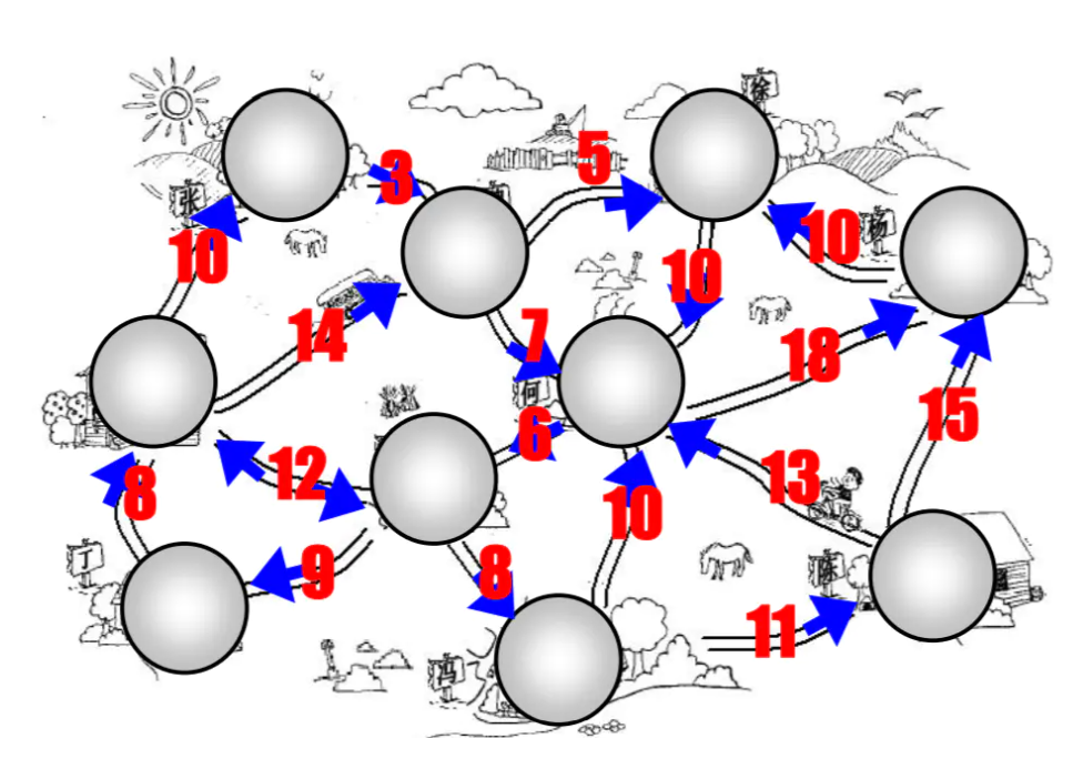
The weighted graph indicates that the edges have a certain weight.
The weight here can be any desired data, such as distance or time spent or ticket price
The following figure is a directed and weighted diagram:
II Representation of Graphs
A graph contains many vertices, as well as vertices and lines (edges) between vertices. These two are very important graph information.
1. vertex representation
The representation of vertices is relatively simple. The vertices above are abstracted into 1 2 3 4, or A B C D. These A, B, C, D can be stored using an array (storing all vertices). Of course, a, B, C and D may also represent data with other meanings (such as the name of the subway station). At this time, another array can be created to store other corresponding data
2. adjacency matrix
The adjacency matrix associates each node with an integer that is used as the subscript value of the array. Use a two-dimensional array to represent the connection between vertices
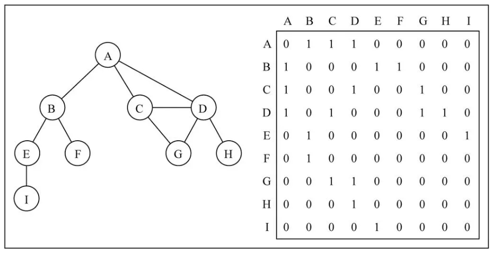
In the two-dimensional array, 0 means no connection and 1 means there is a connection.
Through the two-dimensional array, you can quickly find A vertex and which vertices have connections. (for example, vertex A, you only need to traverse the first row)
In addition, a - A and B - B (that is, the line from the vertex to itself) are usually represented by 0
The problem of adjacency matrix:
If it is an undirected graph, the two-dimensional array displayed by the adjacency matrix is actually a symmetric graph. That is, when a - > D is 1, the symmetrical position D - > 1 must also be 1.
Another serious problem of adjacency matrix is that if the graph is a sparse graph, there will be a large number of zeros in the matrix, which means that computer storage space is wasted to represent non-existent edges. Even if there is only one edge, you must traverse a row to find this edge, which also wastes a lot of time
3. Adjacency table
The adjacency list consists of each vertex in the graph and a list of vertices adjacent to the vertex. This list can be stored in many ways: array / linked list / Dictionary (hash table), etc
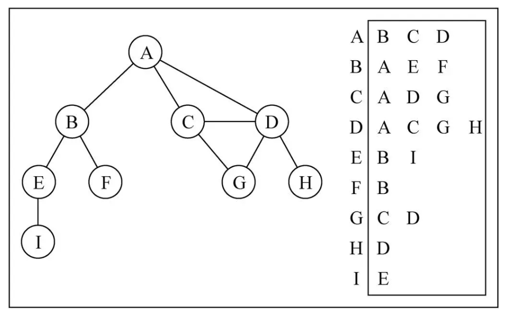
To represent the vertices (edges) associated with vertex A, and A and B/C/D have edges, you can find the corresponding array / linked list / dictionary through A, and then take out the contents.
Adjacency table problem:
The adjacency table is relatively simple to calculate the "out degree" (out degree: point to the number of others, in degree: point to your own number). The adjacency table is troublesome if it is necessary to calculate the "penetration" of a directed graph. An "inverse adjacency table" must be constructed to effectively calculate the "penetration".
III Implementation of graph structure
1. Package diagram structure
    //Package diagram structure
    function Graph(){
        //Attributes: vertex (array) / edge (Dictionary)
        this.vertexes = []  //vertex
        this.edges = new Dictionay()    //edge

    }
Create the constructor of Graph and define two properties:
Vertices: used to store all vertices. We said to use an array to save
adjList: adj is the abbreviation of adj, which means adjacency adjList is used to store all edges in the form of adjacency table
2. How to add vertices
Add some vertices to the graph
    //1. Method of adding vertices
    Graph.prototype.addVertex = function(v){
        this.vertexes.push(v)
        this.edges.set(v,[])
    }
Put the added vertex into the array. In addition, create an array [] for the vertex, which is used to store all the edges connected by the vertex
3. How to add edges
    //2. Method of adding edges
    Graph.prototype.addEdge = function(v1,v2){
        this.edges.get(v1).push(v2)
        this.edges.get(v2).push(v1)
    }
Adding an edge requires two vertices to be passed in, because the edge is an edge between two vertices, and the edge cannot exist alone
Take out the corresponding array according to vertex v and add w to its array
Take out the corresponding array according to vertex w and add v to its array
Here is an undirected graph, so edges can be bidirectional
Test code:
    //Test code
    //1. Create chart structure
    var g = new Graph()
    //2. Add vertex
    var myVertexes = ['A','B','C','D','E','F','G','H','I']
    for(var i=0; i<myVertexes.length; i++){
        g.addVertex(myVertexes[i])
    }
    //3. Add edge
    g.addEdge('A','B')
    g.addEdge('A','C')
    g.addEdge('A','D')
    g.addEdge('C','D')
    g.addEdge('C','G')
    g.addEdge('D','G')
    g.addEdge('D','H')
    g.addEdge('B','E')
    g.addEdge('B','F')
    g.addEdge('E','I')
    //test
    alert(g)
4.toString() method
    //Implement toString method
    Graph.prototype.toString = function(){
        //1. Define the string and save the final result
        var resultString = ''

        //2. Traverse all nodes and edges corresponding to vertices
        for(var i =0; i<this.vertexes.length; i++){
            resultString += this.vertexes[i] + "->"
            var vEdges = this.edges.get(this.vertexes[i])
            for(var j=0; j<vEdges.length; j++){
                resultString += vEdges[j] + ' '
            }
            resultString += '\n'
        }
        return resultString
    }
4, Traversal of Graphs
1. Traversal mode
(1). Ergodic idea of graph
The idea of graph traversal algorithm is to visit each node visited for the first time, and track which vertices have not been accessed. There are two algorithms that can traverse the graph: breadth first search (BFS) and depth first search (DFS)
Both traversal algorithms need to specify the first vertex to be accessed.
(2). Notes on traversal
For each connected vertex that has not been accessed, mark it as discovered and add it to the list of vertices to be accessed. In order to ensure the efficiency of the algorithm, each vertex can be accessed at most twice.
(3). The idea of two algorithms
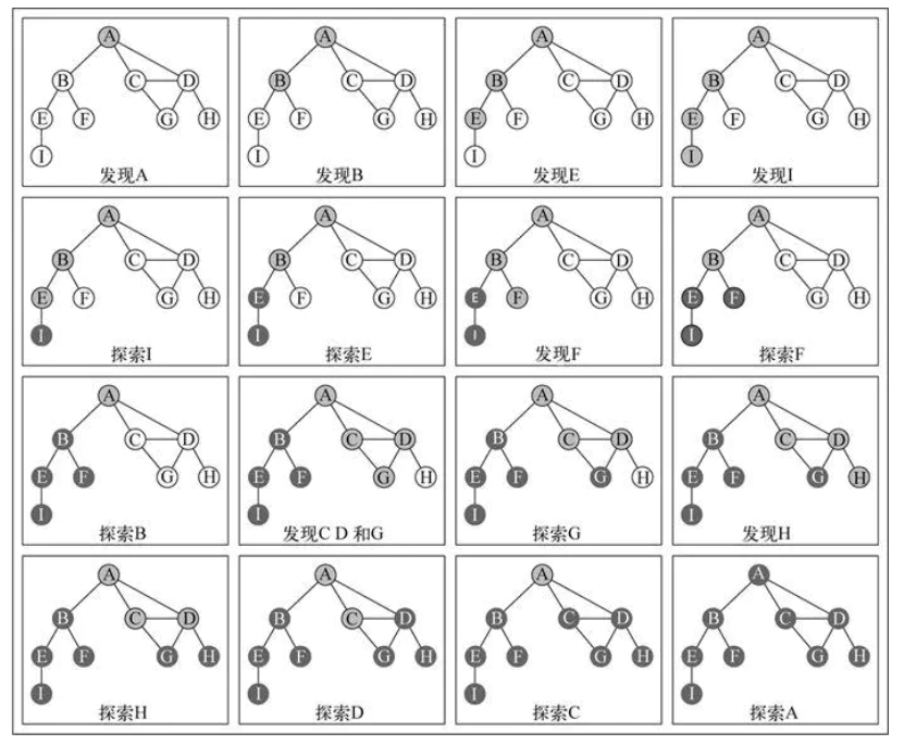
BFS: Based on the queue, the vertices entering the queue are explored first
DFS: Based on the stack, by storing vertices in the stack, vertices are explored along the path, and new adjacent vertices are accessed
In order to record whether vertices have been accessed, we use three colors to reflect their state: (or two colors can also be used)
White: indicates that the vertex has not been accessed
Gray: indicates that the vertex has been visited but not explored
Black: indicates that the vertex has been visited and fully explored
Initialize color code:
    //Initialization status color
    Graph.prototype.initializeColor = function(){
        var colors = []
        for(var i=0; i<this.vertexes.length; i++){
            colors[this.vertexes[i]] = 'white'
        }
        return colors
    }
2. Breadth first search
(1). Idea of breadth first search algorithm
The breadth first algorithm will traverse the graph from the specified first vertex and access all its adjacent points first, just like accessing one layer of the graph at a time. In other words, it is to access vertices from width to depth.
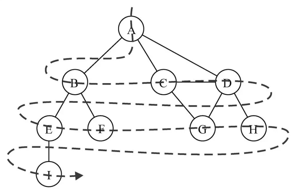
(2). Implementation of breadth first search
    //Achieve breadth first search
    Graph.prototype.bfs = function (initV, handler) {
        //1. Initialize color
        var colors = this.initializeColor()

        //2. Create queue
        var queue = new Queue()

        //3. Add vertices to the queue
        queue.enqueue(initV)

        //4. Loop to fetch elements from the queue
        while (!queue.isEmpty()) {
            //4.1. Take a vertex from the queue
            var v = queue.dequeue()

            //4.2. Gets another vertex connected to the vertex
            var vList = this.edges.get(v)

            //4.3. Set the color of v to gray
            colors[v] = 'gray'

            //4.4 traverse all vertices and join the queue
            for (var i = 0; i < vList.length; i++) {
                var e = vList[i]
                if (colors[e] == 'white') {
                    colors[e] = 'gray'
                    queue.enqueue(e)
                }
            }

            //4.5 access vertex
            handler(v)

            //4.6. Set vertices to black
            colors[v] = 'black'
        }
    }
Test code:
// Call breadth first algorithm
var result = ""
graph.bfs(graph.vertexes[0], function (v) {
    result += v + " "
})
alert(result) // A B C D E F G H I
3. Depth first search
(1). Idea of depth first search
The depth first search algorithm will traverse the graph from the first specified vertex, and follow the path until the path is finally accessed
Then go back and explore a path.
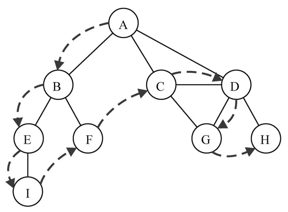
(2). Implementation of depth first search algorithm
The breadth first search algorithm uses queues, which can be completed by stack or recursion. In order to facilitate code writing, recursion is used (recursion is essentially the call of function stack)
    //Depth first search (DFS)
    Graph.prototype.dfs = function(initV,handler){
        //1. Initialize color
        var colors = this.initializeColor()

        //2. Recursive access from a vertex in turn
        this.dfsVisit(initV,colors,handler)
    }
    Graph.prototype.dfsVisit = function(v,colors,handler){
        //1. Set the color to gray
        colors[v] = 'gray'

        //2. Processing v node
        handler(v)

        //3. Access v connected vertices
        var vlist = this.edges.get(v)
        for(var i=0; i < vlist.length; i++){
            var e = vlist[i]
            if(colors[e] == 'white'){
                this.dfsVisit(e,colors,handler)
            }
        }

        //4. Set v to black
        colors[v]='black'
    }
Test code:
    //Call depth first algorithm
    result = ''
    g.dfs(g.vertexes[0],function(v){
        result += v + ' '
    })
    alert(result)
Recursive procedure:
