Lesson 4.3 basic principle and manual implementation of gradient descent

In the previous section, we have successfully constructed the loss function of logistic regression, but due to the particularity of the logistic regression model itself, we cannot adopt the calculation idea similar to SSE when constructing the loss function (at this time, the loss function is not a convex function), so the final loss function cannot be directly solved by the least square method. Of course, this is not just a "problem" of logistic regression model. For most machine learning models, the loss function can not be solved directly by the least square method. At this time, we need to master some optimization methods that can solve the minimum value for more general function forms. In the field of machine learning, the most basic and common method is gradient descent algorithm.

In this section, we will discuss the basic principle and implementation method of gradient descent algorithm in detail, and try to solve the logistic regression loss function on this basis.

# Scientific computing module
import numpy as np
import pandas as pd

# Drawing module
import matplotlib as mpl
import matplotlib.pyplot as plt

# Custom module
from ML_basic_function import *

1, Basic principle of gradient descent and learning rate

1. Data background and least square method

Similar to the maximum likelihood estimation method previously introduced, the gradient descent algorithm itself belongs to a method with relatively complex mathematical theoretical derivation, but the practical application process is not difficult to understand. Therefore, we will start with a simple example and compare it with the calculation process of the least square method to see the general process of gradient descent, and then we will make a more rigorous theoretical derivation.

For example, a simple dataset is represented as follows:

among x x x is the feature of the dataset, y y y is the data set label, assuming that we use simple linear regression y = w x y = wx y=wx to fit this group of data, then we can construct the loss function here as follows:
SSELoss ⁡ ( w ) = ( 2 − 1 ∗ w ) 2 + ( 4 − 2 ∗ w ) 2 + ( 6 − 3 ∗ w ) 2 = w 2 − 4 w + 4 + 4 w 2 − 16 w + 16 + 9 w 2 − 36 w + 36 = 14 w 2 − 56 w + 56 = 14 ( w 2 − 4 w + 4 ) = 14 ( w − 2 ) 2 \begin{aligned} \operatorname{SSELoss}(w) &=(2-1 * w)^{2}+(4-2 * w)^{2}+(6-3 * w)^{2} \\ &=w^{2}-4 w+4+4 w^{2}-16 w+16+9 w^{2}-36 w+36 \\ &=14 w^{2}-56 w+56 \\ &=14\left(w^{2}-4 w+4\right) \\ &=14(w-2)^{2} \end{aligned} SSELoss(w)​=(2−1∗w)2+(4−2∗w)2+(6−3∗w)2=w2−4w+4+4w2−16w+16+9w2−36w+36=14w2−56w+56=14(w2−4w+4)=14(w−2)2​
At this point, the loss function S S E L o s s ( w ) SSELoss(w) Sselos (w) is a unary function about w. To solve the minimum value around the loss function, the least square method can be considered, that is S S E L o s s ( w ) SSELoss(w) The value of sselos (W) derivative function is 0. At this time, there are:
∂ S S E L o s s ( w ) ∂ ( w ) = 28 ( w − 2 ) = 0 \begin{aligned} \frac{\partial S S E L o s s(w)}{\partial(w)} &=28(w-2) \\ &=0 \end{aligned} ∂(w)∂SSELoss(w)​​=28(w−2)=0​
So, w w The optimal solution of w is: w = 2 w=2 w=2
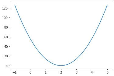
Of course, we can also observe the basic situation of the loss function by drawing an image:

x = np.linspace(-1, 5, 40)
SSELoss = 14 * np.power(x - 2, 2)
plt.plot(x, SSELoss)

2. Basic flow of one-dimensional gradient descent

Of course, around the very simple loss function in the above form, we can also try to use the gradient descent algorithm. Firstly, the goal of the gradient descent algorithm is still to find the minimum value, but different from the least square method, which can directly find the minimum value by solving the equations in one step, the gradient descent algorithm solves the minimum value through an "iterative solution", and its overall solution process can be roughly described as: firstly, randomly select a group of initial values of parameters, and then follow a certain direction, Move to the minimum point step by step. For example:

show_trace(gd(lr = 0.01))
plt.plot(2, 0, 'ro')

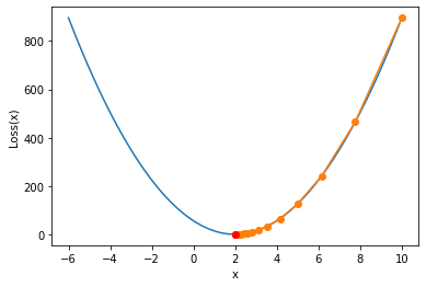
The drawing function of this image will be explained later

2.1 first step of parameter movement

Compared with the above example, we can split the first movement process of parameters into the following three steps:

• Step 1. Randomly select the initial parameter value

In the above example, there is only one parameter. We can set an initial parameter value randomly. For example, we make w 0 = 10 w_0=10 w0​=10.

• Step 2. be based on w 0 w_0 w0, determine the moving direction of the parameter

In the above example, there is only one parameter in the parameter group w w w. Therefore, the parameter changes in only two directions, w w w direction and direction of increase w w w direction of reduction. In gradient descent, the goal of parameter movement is to reduce the value of loss function. Therefore, in the above example, due to w w The initial value of w is 10, so it should be along w w w moves in a reduced direction.

Note that if the loss function contains multiple parameters, there will be multiple change directions of the parameter group. For example, suppose that the parameter group contains two parameters w = ( a , b ) w=(a,b) w=(a,b), then w w The change of w is equivalent to ( a , b ) (a, b) (a,b) the point on this two-dimensional plane moves.

Basic concept of gradient
Of course, in the actual calculation process, we certainly can not determine the moving direction of parameters through observation. In order to determine the moving direction of parameters in more general cases, we need to review the related concepts of gradient vector introduced in Lesson 2. As we mentioned in Lesson 2, let f ( x ) f(x) f(x) is about x x Function of x, where x x x is a vector argument, and x = [ x 1 , x 2 , . . . , x n ] T x = [x_1, x_2,...,x_n]^T x=[x1​,x2​,...,xn​]T
be ∂ f ∂ x = [ ∂ f ∂ x 1 , ∂ f ∂ x 2 , . . . , ∂ f ∂ x n ] T \frac{\partial f}{\partial x} = [\frac{\partial f}{\partial x_1}, \frac{\partial f}{\partial x_2}, ..., \frac{\partial f}{\partial x_n}]^T ∂x∂f​=[∂x1​∂f​,∂x2​∂f​,...,∂xn​∂f​]T
The expression is also called the gradient vector form of vector derivation.
∇ x f ( x ) = ∂ f ∂ x = [ ∂ f ∂ x 1 , ∂ f ∂ x 2 , . . . , ∂ f ∂ x n ] T \nabla _xf(x) = \frac{\partial f}{\partial x} = [\frac{\partial f}{\partial x_1}, \frac{\partial f}{\partial x_2}, ..., \frac{\partial f}{\partial x_n}]^T ∇x​f(x)=∂x∂f​=[∂x1​∂f​,∂x2​∂f​,...,∂xn​∂f​]T
Further, if you assume f ( x ) f(x) f(x) is about parameters x x Loss function of x, then ∇ x f ( x ) \nabla _xf(x) ∇ x ∇ f(x) is the gradient vector or gradient expression of the loss function. And when the parameters of the loss function x x After x selects a set of values, we can calculate the value of the gradient expression, which is also called the gradient of the loss function under a set of parameter values.

For example, in the above example, the loss function f ( w ) = 14 ( w − 2 ) 2 f(w) = 14(w-2)^2 f(w)=14(w−2)2

The gradient vector representation of the loss function is: ∇ w f ( w ) = ∂ f ∂ w = 28 ( w − 2 ) \nabla _wf(w) = \frac{\partial f}{\partial w}=28(w-2) ∇w​f(w)=∂w∂f​=28(w−2)

Specifically, when w 0 = 10 w_0=10 When w0 = 10, the gradient calculation result is ∇ w f ( w 0 ) = 28 ( 10 − 2 ) = 28 ∗ 8 = 224 \nabla _wf(w_0)=28(10-2)=28*8=224 ∇w​f(w0​)=28(10−2)=28∗8=224
After determining the gradient, the moving direction of the parameter is also determined. In the gradient descent algorithm, the moving direction of the parameter is the negative direction of the gradient.

Note that there are two points to note here. One is the negative direction of the gradient. In the above calculation results, 224 is not only the value of the gradient, but also represents the direction of the gradient - the positive direction. At this time, the negative direction of the gradient is the direction of value reduction, which is the same as the observation result of the loss function image. The second is that the parameter moves in the negative direction of the gradient, that is, in the direction of numerical reduction, rather than directly subtracting 224 from the original parameter 10, which is obviously inappropriate.

For a loss function with only one variable, the gradient is the derivative of a point of the function.

• Step 3. Determine the move step and move

After determining the moving direction, it is necessary to further determine the moving distance. In gradient descent, we multiply the gradient by a manually set parameter as the moving distance of each step. This parameter is called step size or Learning rate. For example, in the above case, we can set the Learning rate as lr = 0.01 w 0 w_0 w0# the distance to move is 0.01 ∗ 224 = 2.24 0.01 * 224 = 2.24 0.01 * 224 = 2.24, and it moves towards the negative direction of the gradient, so w 0 w_0 w0# finally moved to w 1 = 10 − 2.24 = 7.76 w_1 = 10-2.24 = 7.76 w1​=10−2.24=7.76

Compared with the step size, it is more appropriate to call the manually set parameter learning rate. This parameter does not represent the real moving distance, but a "ratio" affecting the real moving distance, or the "ratio" of the learning gradient value of the real moving distance.

At this point, the parameters w w w completed the first move, w 0 → w 1 w_0 \rightarrow w_1 w0​→w1​.

2.2 multi round iteration of gradient descent

of course, w w w from w 0 w_0 w0# move to w 1 w_1 w1) in fact, it only moves one step to finally reach the minimum point of the loss function w = 2 w=2 w=2, there is still a long distance, so we need to move many times. Each step in the process of moving parameters many times is actually repeating the above three steps. For example, when we need a second move w w w, the process is as follows:
w 2 = w 1 − l r ⋅ ∇ w f ( w 1 ) w_2 = w_1 - lr \cdot \nabla _wf(w_1) w2​=w1​−lr⋅∇w​f(w1​)
Namely w 2 w_2 w2 equals w 1 w_1 w1 along w 1 w_1 The negative gradient of w1 ， moves l r ⋅ ∇ w f ( w 1 ) lr\cdot\nabla _wf(w_1) Results obtained after lr ⋅ w ∇ f(w1) distance. At this time, we are w 1 w_1 On the basis of w1 ， subtract the learning rate and w 1 w_1 w1 is the product of the gradient.

Of course, and so on, when from w ( n − 1 ) w_{(n-1)} w(n − 1) moves to w n w_n When wn + w n w_n The calculation formula of wn is as follows:
w n = w ( n − 1 ) − l r ⋅ ∇ w f ( w ( n − 1 ) ) w_n = w_{(n-1)} - lr \cdot \nabla _wf(w_{(n-1)}) wn​=w(n−1)​−lr⋅∇w​f(w(n−1)​)
And we can say from w 0 w_0 w0# move to w 1 w_1 w1 ， is the first iteration from w 1 w_1 w1 # move to w 2 w_2 w2 ， is the second iteration from w ( n − 1 ) w_{(n-1)} w(n − 1) moves to w n w_n wn ， is the nth iteration.

Iteration is actually a mathematical concept, which generally refers to the following calculation process: the initial condition of a certain operation is the result of the previous operation, while the result of the current operation is the initial condition of the next calculation.

The algorithm that brings in the gradient value for multiple rounds of iteration and finally makes the value of the loss function gradually decline is called gradient descent.

2. Characteristics and learning rate of gradient descent algorithm

Firstly, we simply verify whether the calculation results of the loss function can be effectively reduced after a series of calculations of the above gradient descent, even if w w w finally approaches the optimal value 2. We can define a function to help us calculate the gradient descent iteration.

def gd(lr = 0.02, itera_times = 20, w = 10):
    """
    Gradient descent calculation function
    :param lr: Learning rate
    :param itera_times: Number of iterations
    :param w: Initial value of parameter
    :return results: List of parameter calculation results for each iteration
    """                              
    results = [w]
    for i in range(itera_times):
        w -= lr * 28 * (w - 2)            # Gradient calculation formula
        results.append(w)
    return results

When we take 0.02 as the learning rate, the initial value is 10 and iterate for 20 rounds, the calculation results of parameters after each round of iteration are as follows:

res = gd()
res
#[10,
# 5.52,
# 3.5488,
# 2.681472,
# 2.29984768,
# 2.1319329792,
# 2.058050510848,
# 2.02554222477312,
# 2.0112385789001728,
# 2.004944974716076,
# 2.0021757888750735,
# 2.0009573471050324,
# 2.000421232726214,
# 2.000185342399534,
# 2.000081550655795,
# 2.00003588228855,
# 2.000015788206962,
# 2.0000069468110633,
# 2.000003056596868,
# 2.000001344902622,
# 2.000000591757154]

We find that the parameter moves towards 2 from 10, and it is very close to the global optimal solution 2 when iterating for 20 rounds. It is also verified here that the gradient descent can indeed help us find the optimal solution. Of course, we can also draw the function images of the above parameter movement process and loss function on a canvas. The specific functions can be realized by the following functions:

def show_trace(res):
    """
    Gradient descent trajectory drawing function
    """
    f_line = np.arange(-6, 10, 0.1)
    plt.plot(f_line, [14 * np.power(x-2, 2) for x in f_line])
    plt.plot(res, [14 * np.power(x-2, 2) for x in res], '-o')
    plt.xlabel('x')
    plt.ylabel('Loss(x)')
show_trace(res)

Next, on this basis, we discuss the basic characteristics of gradient descent algorithm and the general specification of super parameter value in detail.

From the image, we find that the gradient descent calculation process has just begun w w w changes very fast, and as it gradually approaches the minimum point w w The variation range of w decreases gradually, that is, the gradient decline is not an equal step moving process. Of course, according to the formula of gradient descent, w ( n − 1 ) w_{(n-1)} w(n − 1) and w n w_{n} The difference of wn ， is: ∣ w n − w ( n − 1 ) ∣ = ∣ l r ⋅ ∇ w f ( w ( n − 1 ) ) ∣ |w_n - w_{(n-1)}| = |lr \cdot \nabla _wf(w_{(n-1)})| ∣wn​−w(n−1)​∣=∣lr⋅∇w​f(w(n−1)​)∣
And lr is a constant value, that is to say, the gradient value of each point is different (even if the gradient direction is the same), and the closer to the minimum value, the smaller the gradient value. Of course, this can be seen from the gradient calculation formula: ∇ w f ( w ) = ∂ f ∂ w = 28 ( w − 2 ) \nabla _wf(w) = \frac{\partial f}{\partial w}=28(w-2) ∇w​f(w)=∂w∂f​=28(w−2)
Of course, this means that if the gradient value of a point is relatively large, the point should be far from the global minimum. In the process of gradient descent, the moving distance of far point iteration is larger and that of near point iteration is smaller. Of course, when the learning rate corrects the moving distance, the learning rate should not be set too small or too large. For example, when the learning rate is set too small:

plt.subplot(121)
plt.title('lr=0.001')
show_trace(gd(lr=0.001))
plt.subplot(122)
plt.title('lr=0.01')
show_trace(gd(lr=0.01))

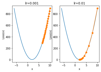
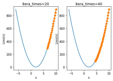
When the learning rate is 0.001, 20 iterations are still far from the minimum point. At this time, we consider further increasing the number of iterations:

plt.subplot(121)
plt.title('itera_times=20')
show_trace(gd(itera_times=20, lr=0.001))
plt.subplot(122)
plt.title('itera_times=40')
show_trace(gd(itera_times=40, lr=0.001))

plt.subplot(121)
plt.title('itera_times=60')
show_trace(gd(itera_times=60, lr=0.001))
plt.subplot(122)
plt.title('itera_times=80')
show_trace(gd(itera_times=80, lr=0.001))

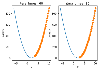
When the learning rate here is 0.001, the number of iterations has increased three times, but it still does not converge to around 2. It takes about 80 iterations to converge to a better effect. However, too many iterations will increase the amount of additional computation, that is, if the learning rate is small, it will consume more computation.

Next, let's look at the possible situation when the learning rate is too large. When we set the learning rate to 0.05, the iterative process is as follows:

plt.subplot(121)
plt.title('lr=0.01')
show_trace(gd(lr=0.01))
plt.subplot(122)
plt.title('lr=0.05')
show_trace(gd(lr=0.05))

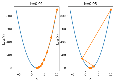
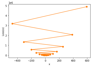
We find that when the learning rate is large, the convergence process is not stable. Of course, small-scale instability does not affect the final convergence result, but the learning rate continues to increase. For example, when we increase the learning rate to 0.08, the overall iterative process of parameters will not converge, but will gradually diverge:

show_trace(gd(lr=0.08))

gd(lr=0.08)
#[10,
# -7.920000000000002,
# 14.300800000000006,
# -13.25299200000001,
# 20.913710080000012,
# -21.45300049920002,
# 31.081720619008028,
# -34.06133356756996,
# 46.71605362378676,
# -53.447906493495594,
# 70.75540405193455,
# -83.25670102439885,
# 107.71830927025458,
# -129.0907034951157,
# 164.55247233394346,
# -199.56506569408992,
# 251.94068146067156,
# -307.92644501123283,
# 386.30879181392874,
# -474.5429018492717,
# 592.9131982930971]

Therefore, it is not difficult to find that the value of learning rate is the key parameter affecting the convergence of the result and the efficient convergence in a finite number of iterations. Too high learning rate will lead to the divergence of results, and too low learning rate will lead to the failure of the model to converge to the optimal result. For more information about the learning rate parameter adjustment strategy, we will introduce it step by step in the subsequent modeling links.

Discussion on the influence of different loss function selection methods or numerical processing methods on the moving distance in the gradient descent process
   what we need to know here is that what affects the iterative convergence result is the real distance of each step, and the real distance of each step is related to the learning rate and gradient. Sometimes we can reduce the gradient in proportion through some numerical processing means, and then the learning rate can be set slightly larger. For example, if we use the MSE calculation formula as the loss function, the gradient calculation formula is changed from the original formula 28 ( w − 2 ) 28(w-2) 28(w − 2) becomes 28 ( w − 2 ) 3 \frac{28(w-2)}{3} 328(w − 2) (three samples in total, M S E = S S E 3 MSE=\frac{SSE}{3} MSE=3SSE​). At this time, it is equivalent to reducing the gradient to the original 1 / 3. When the learning rate remains unchanged, the distance of each movement will also be reduced to the original 1 / 3. In another case, for example, data normalization, that is, a method to adjust the value of the brought in data (described later). If the value brought into the calculation of the loss function is greatly reduced, the final gradient will also be affected and the value will be reduced. At this time, the distance of each movement will also be reduced under the same learning rate.

Moving distance attenuation
In addition, there is another important conclusion here, that is, the farther the parameter point is away from the minimum value point, the gradient of the parameter point is relatively large, and the moving distance of each iteration is relatively large. If the parameter point is closer to the minimum value point, the gradient value is small, and the moving distance of each iteration is relatively small. When it is very close to the minimum value point, the distance of each movement will become very small. Therefore, no matter how many rounds of iterations we add, as long as the parameters do not diverge, the final parameter value point cannot "cross" the minimum value point.

2, General modeling process of gradient descent and multidimensional gradient descent

1. Multidimensional gradient descent and loss function visualization

A more general case is that a model contains multiple parameters, and the loss function is the function composed of these parameters. For example, in Lesson 1, we used simple linear regression with intercept term y = w x + b y=wx+b y=wx+b fit the following data and obtain a loss function with two parameters:

S S E L o s s ( w , b ) = ( y 1 − y ^ 1 ) 2 + ( y 2 − y ^ 2 ) 2 = ( 2 − w − b ) 2 + ( 4 − 3 w − b ) 2 SSELoss(w, b) = (y_1 - ŷ_1)^2 + (y_2 - ŷ_2)^2 = (2 - w - b)^2 + (4 - 3w - b)^2 SSELoss(w,b)=(y1​−y^​1​)2+(y2​−y^​2​)2=(2−w−b)2+(4−3w−b)2
At this time, the loss function image is a three-dimensional image containing two variables

from mpl_toolkits.mplot3d import Axes3D
x = np.arange(-1,3,0.05)
y = np.arange(-1,3,0.05)
w, b = np.meshgrid(x, y)
SSE = (2 - w - b) ** 2 + (4 - 3 * w - b) ** 2

ax = plt.axes(projection='3d')

ax.plot_surface(w, b, SSE, cmap='rainbow')
ax.contour(w, b, SSE, zdir='z', offset=0, cmap="rainbow")  #Generate z-direction projection and project it to the x-y plane
plt.xlabel('w')
plt.ylabel('b')
plt.show()

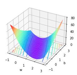
Moreover, we can find out that the global minimum point is (1,1) through the least square method, that is, when w = 1 , b = 1 w=1,b=1 When w = 1 and B = 1, the value of loss function can be minimized. Of course, around this problem, we can also use gradient descent to solve the optimal solution.

2. Gradient descent calculation process

More rigorous steps for gradient descent are given here:

• Step 1. Determine data and model

First, the data and model should be clear, and then the parameters, gradient calculation formula and other variables can be further determined. Here we take y = w x + b y=wx+b y=wx+b simple linear regression is used to fit the above simple data set, and the parameter vector contains two components.

• Step 2. Set initial parameter value

Then we need to select a set of parameter values. A more general method is to assign a set of random numbers to the initial parameters as the initial values. Since the parameter contains two components, the initial value of the parameter vector can be determined by the following process:

np.random.seed(24)
w = np.random.randn(2, 1)                # All parameters are column vectors by default
w
#array([[ 1.32921217],
#       [-0.77003345]])

• Step 3. The gradient expression is obtained according to the loss function

Only when the gradient expression is determined can the gradient be calculated quickly in each subsequent round of iteration. The loss function of linear regression is a loss function constructed around SSE and its derived indicators. Here, MSE is taken as the construction index of loss function, and the calculation can be performed with the help of the defined sselos function.
S S E L o s s ( w ^ ) = ∣ ∣ y − X w ^ ∣ ∣ 2 2 = ( y − X w ^ ) T ( y − X w ^ ) SSELoss(\hat w) = ||y - X\hat w||_2^2 = (y - X\hat w)^T(y - X\hat w) SSELoss(w^)=∣∣y−Xw^∣∣22​=(y−Xw^)T(y−Xw^) M S E L o s s ( w ^ ) = ∣ ∣ y − X w ^ ∣ ∣ 2 2 m = ( y − X w ^ ) T ( y − X w ^ ) m MSELoss(\hat w) = \frac{||y - X\hat w||_2^2}{m} = \frac{(y - X\hat w)^T(y - X\hat w)}{m} MSELoss(w^)=m∣∣y−Xw^∣∣22​​=m(y−Xw^)T(y−Xw^)​
Where m is the total number of training data.

def MSELoss(X, w, y):
    """
    MSE Index calculation function
    """
    SSE = SSELoss(X, w, y)
    MSE = SSE / X.shape[0]
    return MSE

The data is:

features = np.array([1, 3]).reshape(-1, 1)
features = np.concatenate((features, np.ones_like(features)), axis=1)
features
#array([[1, 1],
#       [3, 1]])

labels = np.array([2, 4]).reshape(-1, 1)
labels
#array([[2],
#       [4]])

# SSE when calculating w value
SSELoss(features, w, labels)
#array([[2.68811092]])

# MSE when calculating w value
MSELoss(features, w, labels)
#array([[1.34405546]])

For the gradient expression of linear regression loss function, it can be obtained according to the derivative result of linear regression loss function gradient in Lesson 2: S S E L o s s ( w ^ ) ∂ w ^ = ∂ ∣ ∣ y − X w ^ ∣ ∣ 2 2 ∂ w ^ = ∂ ( y − X w ^ ) T ( y − X w ^ ) ∂ w ^ = ∂ ( y T − w ^ T X T ) ( y − X w ^ ) ∂ w ^ = ∂ ( y T y − w ^ T X T y − y T X w ^ + w ^ T X T X w ^ ) ∂ w ^ = 0 − X T y − X T y + X T X w ^ + ( X T X ) T w ^ = 0 − X T y − X T y + 2 X T X w ^ = 2 ( X T X w ^ − X T y ) = 2 X T ( X w ^ − y ) \begin{aligned} \frac{SSELoss(\hat w)}{\partial{\boldsymbol{\hat w}}} &= \frac{\partial{||\boldsymbol{y} - \boldsymbol{X\hat w}||_2}^2}{\partial{\boldsymbol{\hat w}}} \\ &= \frac{\partial(\boldsymbol{y} - \boldsymbol{X\hat w})^T(\boldsymbol{y} - \boldsymbol{X\hat w})}{\partial{\boldsymbol{\hat w}}} \\ & =\frac{\partial(\boldsymbol{y}^T - \boldsymbol{\hat w^T X^T})(\boldsymbol{y} - \boldsymbol{X\hat w})}{\partial{\boldsymbol{\hat w}}}\\ &=\frac{\partial(\boldsymbol{y}^T\boldsymbol{y} - \boldsymbol{\hat w^T X^Ty}-\boldsymbol{y}^T\boldsymbol{X \hat w} +\boldsymbol{\hat w^TX^T}\boldsymbol{X\hat w})}{\partial{\boldsymbol{\hat w}}}\\ & = 0 - \boldsymbol{X^Ty} - \boldsymbol{X^Ty}+X^TX\hat w+(X^TX)^T\hat w \\ &= 0 - \boldsymbol{X^Ty} - \boldsymbol{X^Ty} + 2\boldsymbol{X^TX\hat w}\\ &= 2(\boldsymbol{X^TX\hat w} - \boldsymbol{X^Ty}) \\ &= 2X^T(X\hat w -y) \end{aligned} ∂w^SSELoss(w^)​​=∂w^∂∣∣y−Xw^∣∣2​2​=∂w^∂(y−Xw^)T(y−Xw^)​=∂w^∂(yT−w^TXT)(y−Xw^)​=∂w^∂(yTy−w^TXTy−yTXw^+w^TXTXw^)​=0−XTy−XTy+XTXw^+(XTX)Tw^=0−XTy−XTy+2XTXw^=2(XTXw^−XTy)=2XT(Xw^−y)​
Here, we use MSE as the loss function, and the gradient expression of the loss function is:
M S E L o s s ( w ^ ) ∂ w ^ = 2 X T ( X w ^ − y ) m \frac{MSELoss(\hat w)}{\partial{\boldsymbol{\hat w}}} = \frac{2X^T(X\hat w -y)}{m} ∂w^MSELoss(w^)​=m2XT(Xw^−y)​

Note: matrix operation can also extract common factors

Therefore, we can define the gradient calculation function of linear regression

def lr_gd(X, w, y):
    """
    Calculation formula of linear regression gradient
    """
    m = X.shape[0]
    grad = 2 * X.T.dot((X.dot(w) - y)) / m
    return grad
# Gradient when calculating w value
lr_gd(features, w, labels)
#array([[-3.78801208],
#       [-2.22321821]])

In fact, this step is also a crucial step in the process of manually realizing gradient descent calculation. As described earlier, only by transforming the equations into matrix form can we make better use of the program for calculation. However, it is worth noting that not all gradient calculations of loss function can be simply expressed in the form of matrix operation.

• Step 4. Perform gradient descent iteration

Given the gradient calculation formula and the initial value of parameters, we can start the gradient descent iterative calculation. In the process of gradient descent, the parameter update refers to the following formula: w n = w ( n − 1 ) − l r ⋅ ∇ w f ( w ( n − 1 ) ) w_n = w_{(n-1)} - lr \cdot \nabla _wf(w_{(n-1)}) wn​=w(n−1)​−lr⋅∇w​f(w(n−1)​)
Then you can define the corresponding function:

def w_cal(X, w, y, gd_cal, lr = 0.02, itera_times = 20):
    """
    Parameter updating function in gradient descent 
    :param X: Training data characteristics
    :param w: Initial parameter value
    :param y: Training data tag
    :param gd_cal: Gradient calculation formula
    :param lr: Learning rate
    :param itera_times: Number of iterations       
    :return w: Final parameter calculation results   
    """
    for i in range(itera_times):
        w -= lr * gd_cal(X, w, y)
    return w

Next, perform gradient descent calculation and iterate for 100 rounds when the learning rate is 0.1:

np.random.seed(24)
w = np.random.randn(2, 1)                # All parameters are column vectors by default
w
#array([[ 1.32921217],
#       [-0.77003345]])

w = w_cal(features, w, labels, gd_cal = lr_gd, lr = 0.1, itera_times = 100)
w
#array([[1.02052278],
#       [0.95045363]])

# SSE when calculating w value
SSELoss(features, w, labels)
#array([[0.0009869]])

# MSE when calculating w value
MSELoss(features, w, labels)
#array([[0.00049345]])

# Gradient when calculating w value
lr_gd(features, w, labels)
#array([[ 0.0070423 ],
#       [-0.01700163]])

We find that the final parameter result approaches the (1,1) point, that is, the overall calculation process can approach the global minimum point after multiple rounds of iteration. The effectiveness of gradient descent itself is also verified. Of course, here is an example of two-dimensional gradient descent. The gradient descent process in higher dimensions is also similar, and the calculation of relevant gradients can be completed with the help of the excellent properties of the array in NumPy.

3. Visual display of two-dimensional gradient descent process

3.1 contour map

In order to facilitate the subsequent display of the properties of other gradient descent algorithms, we observe the movement of parameter points in the process of two-dimensional gradient descent by drawing the contour map of loss function. First, during the above 100 iterations, we can record the calculation results of each iteration:

def w_cal_rec(X, w, y, gd_cal, lr = 0.02, itera_times = 20):
    w_res = [np.copy(w)]
    for i in range(itera_times):
        w -= lr * gd_cal(X, w, y)
        w_res.append(np.copy(w))
    return w, w_res

np.random.seed(24)
w = np.random.randn(2, 1)
w, w_res = w_cal_rec(features, w, labels, gd_cal = lr_gd, lr = 0.1, itera_times = 100)
w_res
#[array([[ 1.32921217],
#        [-0.77003345]]),
# array([[ 1.70801338],
#        [-0.54771163]]),
#       ...
# array([[1.02125203],
#        [0.94869305]]),
# array([[1.02052278],
#        [0.95045363]])]

# Abscissa of all points
np.array(w_res)[:, 0]
#array([[1.32921217],
#       [1.70801338],
#       [1.61908465],
#       ...
#       [1.0220072 ],
#       [1.02125203],
#       [1.02052278]])

• Parameter movement trajectory

Based on this, we can draw the moving tracks of all points in the iterative process on the picture:

plt.plot(np.array(w_res)[:, 0], np.array(w_res)[:, 1], '-o', color='#ff7f0e')

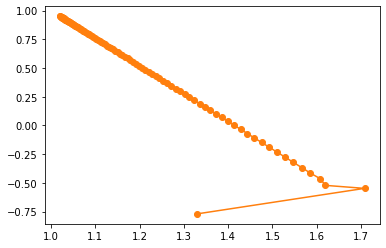
We find that the moving trajectory of the parameter on the parameter plane is not a straight line. Of course, we can also observe the movement of parameter points approaching (1,1) points through contour map.

# Grid point coordinates
x1, x2 = np.meshgrid(np.arange(1, 2, 0.001), np.arange(-1, 1, 0.001))

Where NP Meshgrid generates two sequences. The first sequence is arranged in columns according to the first input parameter, and the second sequence is arranged in rows according to the second input parameter. The output result of this function is mainly used for image rendering with mesh.

np.meshgrid(np.arange(3), np.arange(1, 5))
#[array([[0, 1, 2],
#        [0, 1, 2],
#        [0, 1, 2],
#        [0, 1, 2]]),
# array([[1, 1, 1],
#        [2, 2, 2],
#        [3, 3, 3],
#        [4, 4, 4]])]

# Draw contour map
plt.contour(x1, x2, (2-x1-x2)**2+(4-3*x1-x2)**2)

# Draw the trajectory diagram of parameter point movement
plt.plot(np.array(w_res)[:, 0], np.array(w_res)[:, 1], '-o', color='#ff7f0e')

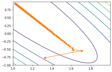
Among them, the contour map requires the input of the range and interval of the grid (i.e. x1 and x2) and the corresponding function relationship (i.e. the function expression of x1 and X2 as independent variables).

3.2 variation diagram of loss function value

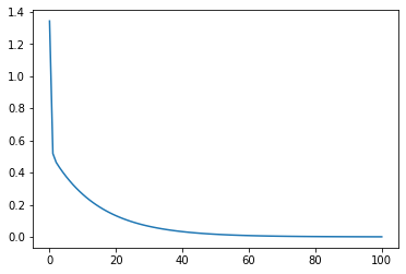
From a more rigorous point of view, we can draw the change curve of its loss function:

loss_value = np.array([MSELoss(features, np.array(w), labels) for w in w_res]).flatten()
loss_value
#array([1.34405546e+00, 5.18623852e-01, 4.63471078e-01, 4.31655465e-01,
#       4.02524386e-01, 3.75373031e-01, 3.50053485e-01, 3.26441796e-01,
#       3.04422755e-01, 2.83888935e-01, 2.64740155e-01, 2.46882992e-01,
#       ...
#       8.62721840e-04, 8.04529820e-04, 7.50262948e-04, 6.99656466e-04,
#       6.52463476e-04, 6.08453732e-04, 5.67412517e-04, 5.29139601e-04,
#       4.93448257e-04])
plt.plot(np.arange(101), loss_value)

It can be found that the loss value decreases strictly in the process of gradient descent. Of course, we can also package the above process into a function:

def loss_vis(X, w_res, y, loss_func):
    loss_value = np.array([loss_func(X, np.array(w), y) for w in w_res]).flatten()
    plt.plot(np.arange(len(loss_value)), loss_value)
# Verify that the function is executable
loss_vis(features, w_res, labels, MSELoss)

4. Gradient descent solution process of linear regression

After mastering the basic principle and properties of gradient descent, we can try to solve the parameters of gradient descent method on the manually created linear regression data set. The linear regression parameters are also solved around the data set in Lesson 3.3, and the gradient descent solution process is still performed according to the above process:

• Step 1. Identify data sets and models

The creation of disturbance items is still small and basically satisfied y = 2 x 1 − x 2 + 1 y=2x_1-x_2+1 y=2x1 − x2 + 1 regular data set.

# Set random number seed
np.random.seed(24)   

# The value of disturbance term is 0.01
features, labels = arrayGenReg(delta=0.01)

• Step 2. Set initial parameters

np.random.seed(24)  
w = np.random.randn(3, 1)
w
#array([[ 1.32921217],
#       [-0.77003345],
#       [-0.31628036]])

• Step 3. Construction of loss function and gradient expression

# SSE when calculating w value
SSELoss(features, w, labels)
#array([[2093.52940481]])

# MSE when calculating w value
MSELoss(features, w, labels)
#array([[2.0935294]])

# Gradient when calculating w value
lr_gd(features, w, labels)
#array([[-1.15082596],
#       [ 0.3808195 ],
#      [-2.52877477]])

• Step 4. Perform gradient descent calculation

Next, the gradient descent parameters are solved with the help of the previously defined parameter update function:

w = w_cal(features, w, labels, gd_cal = lr_gd, lr = 0.1, itera_times = 100)
w
#array([[ 1.99961892],
#       [-0.99985281],
#       [ 0.99970541]])

# SSE when calculating w value
SSELoss(features, w, labels)
#array([[0.09300731]])

# MSE when calculating w value
MSELoss(features, w, labels)
#array([[9.30073138e-05]])

So far, we have completed the manual implementation of the gradient descent algorithm.

3, Evaluation of gradient descent algorithm

1. Advantages of gradient descent algorithm

In this section, we use the loss function of linear regression to construct a gradient expression to calculate the gradient descent. Although the loss function of linear regression can be solved directly by the least square method, the gradient descent algorithm still has certain advantages in some scenarios. These advantages are mainly reflected in two aspects. One is compared with large-scale numerical matrix operation, The iterative solution followed by gradient descent is more efficient (although large-scale matrix operation can also reduce the amount of data calculated at each time by dividing the block matrix). The second is that gradient descent can still effectively find the minimum point (or solution space) when some least squares methods cannot calculate the only optimal solution in the whole domain.

Numerical and analytical solutions
For the results calculated by strict mathematical formula, similar to the results calculated by the least square method, it is also called analytical solution. The results obtained by a certain calculation method or calculation process, such as the results of gradient descent, are also called numerical solutions.

2. Limitations of gradient descent algorithm

However, the gradient descent algorithm still has some limitations. When the loss function is not convex, that is, there may be a local minimum or saddle point, the gradient descent may not be able to accurately find the global minimum.

2.1 local minimum trap

The so-called local minimum value means that the values at the left and right ends of the point are greater than the point, but the point is not the global minimum value point. For example, function: f ( x ) = x ⋅ c o s ( π x ) f(x)=x\cdot cos(\pi x) f(x)=x⋅cos(πx)
The function image is as follows:

x = np.arange(-1, 2, 0.1)
y = x * np.cos(np.pi * x)
fig = plt.plot(x, y)[0]
fig.axes.annotate('local minimun', xytext=(-0.77, -1), 
                  arrowprops=dict(arrowstyle='->'), xy=(-0.3, -0.25))
fig.axes.annotate('global minimun', xytext=(0.6, 0.8), 
                  arrowprops=dict(arrowstyle='->'), xy=(1.1, -0.95))
plt.xlabel('x')
plt.ylabel('x·cos(pi·x)')

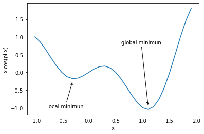
Note, where PLT Plot (x, y) [0] is the returned image object, axes Annotate is to add text or graphics to the image, xytext is the text start coordinate, and xy is the graphics start coordinate.

According to the distance attenuation theory of gradient descent introduced earlier, since the gradient of the local minimum point is also zero, if the parameter point falls into the local minimum, it is impossible to cross the local minimum to reach the global minimum point. hypothesis f ( x ) = x ⋅ c o s ( π x ) f(x)=x\cdot cos(\pi x) f(x)=x ⋅ cos(π x) is the loss function at this time, and there is a unique parameter x at this time, then the gradient descent iterative calculation has the following process.

Note: Here we directly give the loss function when the data, model and evaluation index are unknown.

The first is the process from the loss function to the gradient calculation expression. Since the loss function has only one parameter, the gradient expression is f ′ ( x ) = ( x ⋅ c o s ( π x ) ) ′ = c o s ( π x ) + x ⋅ ( − s i n ( π x ) ) ⋅ π f'(x) = (x\cdot cos(\pi x))' = cos(\pi x) + x\cdot (-sin(\pi x)) \cdot \pi f′(x)=(x⋅cos(πx))′=cos(πx)+x⋅(−sin(πx))⋅π
We can define the function expression and derivative function expression of the function.

def f_1(x):
    return (x*np.cos(np.pi*x))
f_1(-1)
#1.0

def f_gd_1(x):
    return (np.cos(np.pi*x)-x*np.pi*(np.sin(np.pi*x)))
f_gd_1(-1)
#-1.0000000000000004

And the corresponding gradient update function

def gd_1(lr = 0.02, itera_times = 20, w = -1):
    """
    Gradient descent calculation function
    :param lr: Learning rate
    :param itera_times: Number of iterations
    :param w: Initial value of parameter
    :return results: List of parameter calculation results for each iteration
    """                              
    results = [w]
    for i in range(itera_times):
        w -= lr * f_gd_1(w)              # Gradient calculation formula
        results.append(w)
    return results

When we take 0.02 as the learning rate, the initial value of the parameter is - 1 and iterate for 5000 rounds, the calculation results of the parameters after each round of iteration are as follows:

res = gd_1(itera_times = 5000)
res[-1]
#-0.2738526868008511

We find that the parameters finally stay near -0.27. Of course, for the above one-dimensional gradient descent, we can also draw the trajectory diagram corresponding to the change of parameters for observation.

def show_trace_1(res):
    """
    Gradient descent trajectory drawing function
    """
    f_line = np.arange(-1, 2, 0.01)
    plt.plot(f_line, [f_1(x) for x in f_line])
    plt.plot(res, [f_1(x) for x in res], '-o')
    plt.xlabel('x')
    plt.ylabel('Loss(x)')

show_trace_1(res)

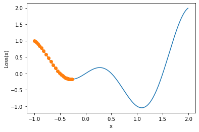
We find that the parameter finally stays near the local minimum and cannot cross the local minimum. According to the gradient descent moving distance attenuation theory introduced earlier, the gradient at this point should also be a value tending to 0 after 5000 rounds of final iteration. Of course, this is also in line with the characteristics of local minimum, and the derivative is 0.

f_gd_1(res[-1])
#-1.2212453270876722e-15

Of course, for the local minimum trap of gradient descent, the fundamental reason is that the distance of parameter movement in the process of gradient descent is directly linked to the gradient. This characteristic of gradient descent not only leads to the local minimum trap, but also another more common trap - saddle point trap.

2.2 saddle point trap

First, let's look at what a saddle point is. Saddle points have many rigorous academic definitions. Simply understand that saddle points are those points that are not extreme points but have a gradient of 0. The so-called extremum refers to those points where the upper derivative of a continuous function is 0 and the monotonicity of all sides is opposite. Extremum includes local minimum, minimum, local maximum and maximum. The difference between saddle point and extreme point is that the derivative is 0, and the monotonicity of the left and right sides is the same, for example:
f ( x ) = x 3 f(x)=x^3 f(x)=x3
We observe the saddle point by drawing the function image of the function.

x = np.arange(-2, 2, 0.1)
y = np.power(x, 3)

fig = plt.plot(x, y)[0]
fig.axes.annotate('saddle point', xytext=(-0.52, -5), 
                  arrowprops=dict(arrowstyle='->'), xy=(0, -0.2))
plt.xlabel('x')
plt.ylabel('x**3')

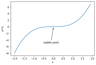
Further, we look at how the lower saddle point affects the gradient descent process. The first is the process from loss function to gradient calculation expression. Since the loss function has only one parameter, the gradient expression is:
f ′ ( x ) = 3 x 2 f'(x) = 3x^2 f′(x)=3x2
We can define the function, the derivative function and the trajectory drawing function

# x**3 function
def f_2(x):
    return np.power(x, 3)
f_2(-1)
#-1

# x**3 derivative
def f_gd_2(x):
    return (3*np.power(x, 2))
f_gd_2(-1)
#3

# Gradient update function
def gd_2(lr = 0.05, itera_times = 200, w = 1):
    """
    Gradient descent calculation function
    :param lr: Learning rate
    :param itera_times: Number of iterations
    :param w: Initial value of parameter
    :return results: List of parameter calculation results for each iteration
    """                              
    results = [w]
    for i in range(itera_times):
        w -= lr * f_gd_2(w)              # Gradient calculation formula
        results.append(w)
    return results

When we take 0.05 as the learning rate, the initial value of the parameter is 1 and iterate for 5000 rounds, the calculation results of the parameters after each round of iteration are as follows:

res = gd_2(itera_times=5000)
res[-1]
#0.0013297766246039373

def show_trace_2(res):
    """
    Gradient descent trajectory drawing function
    """
    f_line = np.arange(-1, 2, 0.01)
    plt.plot(f_line, [f_2(x) for x in f_line])
    plt.plot(res, [f_2(x) for x in res], '-o')
    plt.xlabel('x')
    plt.ylabel('Loss(x)')
    
show_trace_2(res)

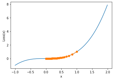
Similarly, the gradient descent cannot reach the point with smaller value across the saddle point, and we judge that the gradient of the parameter point is very small after 5000 iterations:

f_gd_2(res[-1])
#5.304917614029122e-06

We can draw a two-dimensional image containing saddle points for observation:

x, y = np.mgrid[-1:1:31j,-1:1:31j]
z = x**2- y**2
ax = plt.axes(projection='3d')
ax.plot_wireframe(x, y, z,**{'rstride':2,'cstride':2})
ax.plot([0],[0],[0],'rx')
ticks =[-1,0,1]
plt.xticks(ticks)
plt.yticks(ticks)
ax.set_zticks(ticks)
plt.xlabel('x')
plt.ylabel('y')

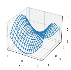
Note that in practice, the frequency of saddle point is higher than the local minimum point.

3. Essence and improvement method of gradient descent algorithm

According to the discussion of local minimum and saddle point, it is not difficult to find that the essential function of gradient descent is to move the parameter point to the point with gradient 0. When the loss function is a strictly convex function, the point with gradient 0 is the global minimum point. However, if the loss function is not a convex function, the point with gradient 0 may be a local minimum point or saddle point. At this time, the gradient descent cannot move out of the local minimum point or saddle point because the gradient is 0. Although the loss functions of most linear models are convex functions, the loss functions constructed by many complex machine learning models are not necessarily strictly convex functions. In order to avoid local minimum point or saddle point traps, we must improve the gradient descent algorithm. One of the most basic and general improvement methods is to substitute a small part of data each time when building the loss function, so as to give the parameters a chance to jump out of the trap, which is the so-called random gradient descent and small batch gradient descent. We will discuss the calculation process and practical effect of these two improved methods in detail in the next class.

Lesson 4.4 random gradient descent and small batch gradient descent

In the previous section, we talked about the calculation process and algorithm characteristics of gradient descent algorithm, from which we know that gradient descent can finally converge to a point with gradient of 0 through multiple rounds of iterative calculation. When the loss function is convex, because the global minimum point is the only point with gradient of 0, the gradient descent can converge to the global minimum smoothly. However, if the loss function is not convex, the gradient descent algorithm is easy to fall into the local minimum point trap or saddle point trap. At this point, we need to consider "improving" the original algorithm. There are many ways to improve the gradient descent algorithm, among which the simplest and effective way is to adjust the number of samples brought into training each time, and avoid the trap of "non global minimum but gradient is 0" through the inconsistency of local laws. Of course, under the basic idea of adjusting the number of samples brought in each time, two algorithms are derived according to the actual amount of data brought in - random gradient descent and small batch gradient descent.

# Scientific computing module
import numpy as np
import pandas as pd

# Drawing module
import matplotlib as mpl
import matplotlib.pyplot as plt

# Custom module
from ML_basic_function import *

1, Theoretical basis of loss function

Firstly, we need to supplement some relevant theories about loss function.

• Different training data, loss function and model parameters are different

There is a simple but often forgotten fact, that is, the loss function will be different with different training data, and then the trained model parameters will be different, that is, different model results will be obtained finally. For example, there are data sets as follows:

And we use a simple linear regression equation without intercept term for fitting: y = w x y=wx y=wx
At this time, the calculation formula of loss function is: M S E L o s s ( w ) = ∑ i = 1 n ∣ ∣ y i − y ^ i ∣ ∣ 2 2 n MSELoss(w)=\frac{\sum_{i=1}^n||y_i-\hat y_i||_2^2}{n} MSELoss(w)=n∑i=1n​∣∣yi​−y^​i​∣∣22​​
When we bring in all four data for calculation, the loss function is:
Loss ⁡ 4 ( w ) = ( 2 − w ) 2 + ( 5 − 3 w ) 2 + ( 4 − 6 w ) 2 + ( 3 − 8 w ) 2 4 = 110 w 2 − 130 w + 54 4 \begin{aligned} \operatorname{Loss}_{4}(w) &=\frac{(2-w)^{2}+(5-3 w)^{2}+(4-6 w)^{2}+(3-8 w)^{2}}{4} \\ &=\frac{110 w^{2}-130 w+54}{4} \end{aligned} Loss4​(w)​=4(2−w)2+(5−3w)2+(4−6w)2+(3−8w)2​=4110w2−130w+54​​
Correspondingly, we can get the optimal solution by solving the loss function w w w result, let the derivative of the loss function be 0 w = 100 220 = 5 11 w=\frac{100}{220}=\frac{5}{11} w=220100 = 115, the model is finally solved y = 5 11 x y = \frac{5}{11}x y=115​x

If we bring in one piece of data for calculation, such as the first piece of data for calculation, the loss function calculation formula is:
L o s s 1 ( w ) = ( 2 − w ) 2 = w 2 − 4 w + 4 Loss_1(w)=(2-w)^2 = w^2-4w+4 Loss1​(w)=(2−w)2=w2−4w+4
At this time, the optimal parameter result is w = 2 w=2 w=2, that is, the training model is y = 2 x y=2x y=2x. Obviously, the training data are different, the loss function is different, and the training model is also different.

• Loss function is actually an embodiment of the law of data set

Because the model is actually the embodiment of the law of the data set, and the loss function is the basic function for solving the model parameters, we can believe that the loss function is actually an embodiment of the law shown by a batch of data, and the loss functions of different data are different, so we believe that the basic laws corresponding to these batches of data are different. If the forms of the above two loss functions are different, it means that the basic laws of the data behind them are different.

• The law is consistent and the loss function is also consistent

However, we also need to know that sometimes the data seem different, but the laws behind them are consistent. At this time, the loss function is also consistent. In principle, the loss function is an equation guiding the solution of the global minimum. If multiple (partial) data laws are consistent, the constructed loss function will be basically consistent, at least the global minimum point will be consistent. For example, the following two data laws are consistent, which are satisfied y = 2 x y=2x The basic law of y=2x

Then the loss function is constructed around these two data respectively, and the following results can be obtained:
M S E L o s s ( w ) 1 = ( 2 − w ) 2 MSELoss(w)_1 = (2-w)^2 MSELoss(w)1​=(2−w)2 M S E L o s s ( w ) 2 = ( 4 − 2 w ) 2 = 4 ( 2 − w ) 2 MSELoss(w)_2 = (4-2w)^2 = 4(2-w)^2 MSELoss(w)2​=(4−2w)2=4(2−w)2
Although the coefficient difference between the two loss functions seems to be in proportion, this difference does not affect the calculation process of the actual gradient decline, as described above M S E L o s s 1 MSELoss_1 MSELoss1} and M S E L o s s 2 MSELoss_2 The proportional difference of MSELoss2 ＾ can be completely consistent with the final parameter iteration process by setting a negative proportional learning rate in the iteration process. For example, we can make the initial w w If w is 0, the iterative process of the two loss functions is as follows:

# Create first data
x1 = np.array([[1]])
y1 = np.array([[2]])
w1 = np.array([[0.]])

# Calculate w1 current gradient
lr_gd(x1, w1, y1)
#array([[-4.]])

# Create second data
x2 = np.array([[2]])
y2 = np.array([[4]])
w2 = np.array([[0.]])
# Calculate w2 current gradient
lr_gd(x2, w2, y2)
#array([[-16.]])

Then, the gradient descent iterative operation process under the loss function created by the first data can be calculated

w_cal_rec(x1, w1, y1, gd_cal = lr_gd, lr = 0.1, itera_times = 10)
#(array([[1.78525164]]),
# [array([[0.]]),
#  array([[0.4]]),
#  array([[0.72]]),
#  array([[0.976]]),
#  array([[1.1808]]),
#  array([[1.34464]]),
#  array([[1.475712]]),
#  array([[1.5805696]]),
#  array([[1.66445568]]),
#  array([[1.73156454]]),
#  array([[1.78525164]])])

Then iterate for 10 rounds, reduce the learning rate to 1 / 4, and calculate the gradient descent iterative process under the loss function constructed by the second data

w_cal_rec(x2, w2, y2, gd_cal = lr_gd, lr = 0.025, itera_times = 10)
#(array([[1.78525164]]),
# [array([[0.]]),
#  array([[0.4]]),
#  array([[0.72]]),
#  array([[0.976]]),
#  array([[1.1808]]),
#  array([[1.34464]]),
#  array([[1.475712]]),
#  array([[1.5805696]]),
#  array([[1.66445568]]),
#  array([[1.73156454]]),
#  array([[1.78525164]])])

It is not difficult to find that the two are exactly the same. In other words, the proportional difference of the loss function can be completely eliminated by the learning rate, which is a manually set parameter. Therefore, in this sense, the loss function created by the same law and different data is essentially the "same" loss function. Of course, if we construct a loss function jointly constructed by these two data at this time, the loss function is also consistent with the above two loss functions.

It is worth noting that this characteristic of loss function will also be the fundamental factor affecting the effectiveness of random gradient descent or small batch gradient descent.

So far, let's look back at the first section L o s s ( w ) 4 Loss(w)_4 Loss(w)4} and L o s s ( w ) 1 Loss(w)_1 Loss(w)1, the reason why they are different is because L o s s ( w ) 4 Loss(w)_4 The four data behind Loss(w)4 ， show the overall law and M S E L o s s ( w ) 1 MSELoss(w)_1 The rule shown by a piece of data on the back of mselos (W) 1 ， is inconsistent.
Loss ⁡ 4 Data set behind \operatorname{Loss}_{4} \text {dataset behind} Data set behind Loss4 #

L o s s 4 ( w ) = 110 w 2 − 130 w + 54 4 Loss_4(w) =\frac{110w^2-130w+54}{4} Loss4​(w)=4110w2−130w+54​
Loss ⁡ 1 Data set behind \operatorname{Loss}_{1} \text {dataset behind} The dataset behind Loss1 #
L o s s 1 ( w ) = ( 2 − w ) 2 = w 2 − 4 w + 4 Loss_1(w)=(2-w)^2 = w^2-4w+4 Loss1​(w)=(2−w)2=w2−4w+4

• Local law and overall law

In order to facilitate the distinction, we call the law shown by the training data set as the overall law of the training data, and the law shown by a single piece or several pieces of data as the local law. For dataset 1, the local laws of the first data are inconsistent with those of the whole dataset, while for dataset 2, the laws of the first data, the second data and the whole dataset are consistent. In addition, we also call part of the data in the training data set as the sub data set of the training data.

However, in most of the actually obtained data, due to various errors, it is difficult to have multiple data laws completely consistent like data set 2. In most cases, there are certain law differences in the sub data sets of the training data set, not only between different sub data sets, Moreover, there are some regular differences between the sub data set and the training data set as a whole.

• Relative unity of local law and overall law

Although the local law and the overall law are not consistent, the local law and the overall law are relatively unified. For example, we still take dataset 1 as an example, and the first loss function is constructed from the previous two data L o s s 2 Loss_2 Loss2. Construct another loss function from the last two data L o s s 3 Loss_3 Loss3, the loss function is calculated as follows:

Loss ⁡ 2 = ( 2 − 1 w ) 2 + ( 5 − 3 w ) 2 2 = w 2 − 4 w + 4 + 9 w 2 − 30 w + 25 2 = 10 w 2 − 34 w + 29 2 Loss ⁡ 3 = ( 4 − 6 w ) 2 + ( 3 − 8 w ) 2 2 = 36 w 2 − 48 w + 16 + 64 w 2 − 48 w + 9 2 = 100 w 2 − 96 w + 25 2 \begin{aligned} \operatorname{Loss}_{2} &=\frac{(2-1 w)^{2}+(5-3 w)^{2}}{2} \\ &=\frac{w^{2}-4 w+4+9 w^{2}-30 w+25}{2} \\ &=\frac{10 w^{2}-34 w+29}{2} \\ \operatorname{Loss}_{3} &=\frac{(4-6 w)^{2}+(3-8 w)^{2}}{2} \\ &=\frac{36 w^{2}-48 w+16+64 w^{2}-48 w+9}{2} \\ &=\frac{100 w^{2}-96 w+25}{2} \end{aligned} Loss2​Loss3​​=2(2−1w)2+(5−3w)2​=2w2−4w+4+9w2−30w+25​=210w2−34w+29​=2(4−6w)2+(3−8w)2​=236w2−48w+16+64w2−48w+9​=2100w2−96w+25​​
At this time, the overall loss function is actually the average of the above two:
L o s s 4 ( w ) = 110 w 2 − 130 w + 54 4 Loss_4(w) =\frac{110w^2-130w+54}{4} Loss4​(w)=4110w2−130w+54​
Therefore, we can understand it as: the loss function representing the local law can also partially represent the overall loss function.

A more rigorous expression is that the loss function of the local law is, on average, a good estimate of the overall loss function.

Of course, local laws are relatively unified with each other.

• Improvement of gradient descent calculation process

Therefore, we can further discuss the improvement idea of gradient descent.

In short, each parameter movement in the gradient descent process is based on the overall law (the loss function corresponding to all data sets) for each parameter iteration, whether it is Stochastic Gradient Descent or mini Batch Gradient Descent, In fact, they all use the local law (loss function of some data) to carry out each parameter iteration. For random gradient descent, one piece of data is selected for each parameter iteration to build the loss function, while for small Batch Gradient Descent, one small batch of data (subset of training data set) is selected for each iteration. For example, a total of 100 data are divided into 10 subsets, Each subset contains 10 pieces of data, and then the loss function brought into one subset for each gradient descent is calculated. According to this division method, the original gradient descent algorithm is also called BGD (Batch Gradient Descent). Of course, it is not difficult to find that both SGD and BGD are special cases of small Batch Gradient Descent, that is, in small Batch Gradient Descent, when the subset is equal to the full set, the small Batch Gradient Descent is BGD, and when each subset has only one data, the small Batch Gradient Descent is SGD.

It is worth noting that in some deep learning computing frameworks (such as PyTorch), small batch gradient descent is also classified as SGD.

This modification idea itself is not difficult to understand, but how to optimize the gradient descent process and make it jump out of the local minimum point? How does the inconsistency of local laws play a role in this process? This requires us to go deep into the specific calculation process of random gradient descent and small batch gradient descent for observation.

Briefly summarize the above theoretical basis:
1. The data law can be expressed by loss function. Different forms of loss function represent different data laws behind the loss function;
2. Generally speaking, for a data set, there are some differences between local laws and between local laws and overall laws, but there is also some unity;
3. Using the characteristic of "unity of opposites" between local laws, we can change the direction of parameter movement in the process of parameter movement, so as to avoid local minimum or saddle point trap.

2, Stochastic Gradient Descent

1. Calculation flow of random gradient descent

First, let's discuss the calculation process of SGD and the precautions in the use process. Let's start with a simple example and assume that the existing data sets are as follows:

At this time, if we use SGD to update and iterate the parameter points, we extract one piece of data each time to construct the loss function, and then calculate it. Similarly, we construct a simple linear regression without intercept term y = w x y=wx y=wx for modeling, then the loss function of the first data is: L o s s 1 ( w ) = ( 2 − w ) 2 Loss_1(w) = (2-w)^2 Loss1​(w)=(2−w)2
The loss function of the second data is L o s s 2 ( w ) = ( 5 − 3 w ) 2 Loss_2(w)=(5-3w)^2 Loss2​(w)=(5−3w)2
In the actual SGD execution process, we will first disorder the data set, and then select the loss function of each data in turn for parameter update calculation. Of course, if the training set and test set are randomly segmented, there is no need to carry out disorder processing again. Now it is assumed that the above data is the result of disorder processing, given the initial parameters w 0 = 0 w_0=0 When w0 = 0, we can iterate the parameters according to the following process. First, we define the parameters and data

w = 0
x = np.array([[1], [3]])
x
#array([[1],
#       [3]])
y = np.array([[2], [5]])
y
#array([[2],
#       [5]])

Then the first round of iteration can be started, and the first data is brought in to modify the parameters for the first time. The actual calculation process is equivalent to modifying the parameters with the help of the gradient calculated by the loss function of the first data. The process is as follows:

# Perform the first iteration
w = w_cal(x[0], w, y[0], lr_gd, lr = 0.02, itera_times = 1)
w
#0.08

Then, the loss function gradient of the second data is used to modify the parameters for the second time

# Perform the second iteration
w = w_cal(x[1], w, y[1], lr_gd, lr = 0.02, itera_times = 1)
w
#0.6512

Contrast gradient descent calculation process

w = 0
w_cal(x, w, y, lr_gd, lr = 0.02, itera_times = 2)
#array([[0.612]])

So far, we have performed a total of two rounds of iterations, and the parameters have moved two steps. All the data has only the number of pieces. Two rounds of iterations just use one round of all the data. At this time, we call it iterative one round of epoch, that is, the gradient descent process traverses the data. In the process of random gradient descent and small batch gradient descent, we generally use epoch index to explain the current iteration progress. Next, we try to iterate over 40 epochs.

w = 0
epoch = 40

for j in range(epoch):
    for i in range(2):
        w = w_cal(x[i], w, y[i], lr_gd, lr = 0.02, itera_times = 1)
# Final parameter value
w
#1.6887966746685015

Of course, we can also define the above process as a function:

def sgd_cal(X, w, y, gd_cal, epoch, lr = 0.02):
    """
    Random gradient descent calculation function
    :param X: Training data characteristics
    :param w: Initial parameter value
    :param y: Training data tag
    :param gd_cal: Gradient calculation formula
    :param epoch: Number of traversal data sets
    :param lr: Learning rate      
    :return w: Final parameter calculation results       
    """
    m = X.shape[0]
    n = X.shape[1]
    for j in range(epoch):
        for i in range(m):
            w = w_cal(X[i].reshape(1, n), w, y[i].reshape(1, 1), gd_cal=gd_cal, lr=lr, itera_times = 1)
    return w

Verify function output

w = 0
sgd_cal(x, w, y, lr_gd, epoch=40, lr=0.02)
#array([[1.68879667]])

So, is 1.688 the global minimum? At this time, we can also compare the gradient descent with the results calculated around the above problem:

# Gradient descent calculation process
w = 0
w = w_cal(x, w, y, lr_gd, lr = 0.02, itera_times = 100)
w
#array([[1.7]])

The overall loss function is L o s s ( w ) = w 2 − 4 w + 4 + 9 w 2 − 30 w + 25 = 10 w 2 − 34 w + 29 Loss(w)=w^2-4w+4+9w^2-30w+25=10w^2-34w+29 Loss(w)=w2−4w+4+9w2−30w+25=10w2−34w+29
The corresponding gradient calculation formula is ∇ w L o s s ( w ) = 20 w − 34 \nabla _wLoss(w)=20w-34 ∇w​Loss(w)=20w−34
Therefore, the global minimum point should be w = 34 20 = 1.7 w=\frac{34}{20}=1.7 w=2034​=1.7
In other words, although the random gradient descent is effective, it can not converge to the global optimal solution like the batch gradient descent, and the random gradient descent can only converge near the global minimum point. To find out the reasons behind this and find out the optimization method, we need to further explore the characteristics of random gradient descent algorithm.

2. Algorithm characteristics of random gradient descent

• Oscillation characteristics of iteration results

Although from the perspective of execution process, SGD only changed "bring in all data for calculation every time" of gradient descent to "bring in one data for calculation every time", in fact, this will greatly affect the direction of each movement of parameters, so that the parameters can not converge to the global optimal solution in the end, But at the same time, it also makes the parameter iteration process cross the local minimum point.

We also review the iterative process of parameters in the above example. In the first iteration of the first round of epoch, the parameter point starts from 0, and actually advances according to the minimum value point of the loss function of the first data. The loss function and image of the first data are as follows: L o s s 1 ( w ) = ( 2 − w ) 2 Loss_1(w) = (2-w)^2 Loss1​(w)=(2−w)2

x1 = np.arange(1.5, 2.5, 0.01)
y1 = np.power(2-x1, 2)
plt.plot(x1, y1)

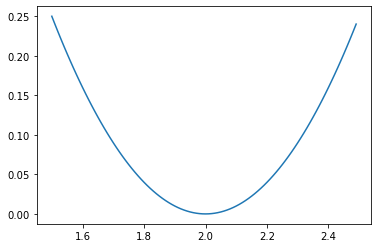
That is, towards w = 2 w=2 w=2 is going forward at this point. In the second iteration, the parameter points move towards the minimum value of the loss function corresponding to the second data. The loss function and image of the second data are as follows: L o s s 2 ( w ) = ( 5 − 3 w ) 2 Loss_2(w)=(5-3w)^2 Loss2​(w)=(5−3w)2

y2 = np.power(5-3*x1, 2)
plt.plot(x1, y1, label='x1')
plt.plot(x1, y2, label='x2')
plt.legend(loc = 1)

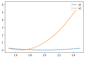
The minimum point of the second data loss function is 5 3 = 1.667 \frac{5}{3}=1.667 35 = 1.667, the minimum point of the loss function of the two data is not consistent, and the global minimum point is between 1.667 and 2. Therefore, in the actual iterative process, when the parameter point is located to the left of the two minimum points, that is, when the parameter is less than 1.667, no matter which data loss function is followed for gradient descent, it can move towards the global minimum point. However, when the parameter points are iterated between 1.667 and 2, the parameter iteration will fall into a "dilemma". When the first data is brought in for gradient descent, the algorithm execution process will require the parameter points to retreat to the point of 1.667; If the second data is brought in for gradient descent, the algorithm execution process will require the parameter point to move forward to 2. We can observe the moving process of parameter points in detail.

Different loss functions "require" different iteration directions.

w = 0
epoch = 40
for j in range(epoch):
    for i in range(2):
        w = w_cal(x[i], w, y[i], lr_gd, lr = 0.02, itera_times = 1)
        print(w)
#0.08
#0.6512
#0.705152
#1.05129728
#...
#1.6887966710099307
#1.7012448041695334
#1.6887966746685015

• Results oscillation and escape from local minimum points

We find that the final parameter fluctuates back and forth between 1.7 and 1.68, which is a "dilemma". Before considering how to improve this problem, let's take a look at the impact of the uncertain direction of this parameter point in the iterative process. From the above iterative process of w, we find that the inconsistency of parameter direction occurs when the parameter is located between two minimum points, which is not affected by the global minimum point 1.7, or "not" by the point where the gradient of the overall loss function is 0. Then we reasonably speculate that there may be a case that the global loss function has a local minimum, but the gradient of a data at that point is not 0. Then, when the parameter iterates to the global local minimum point, the data is just brought in for gradient descent. Because the gradient of the data at this point is not 0, the parameter will cross the local minimum point smoothly. Suppose the loss function of all training data is y = x ⋅ c o s ( π x ) y=x\cdot cos(\pi x) y=x ⋅ cos(π x), and the loss function of a data is y = ( x − 0.7 ) 2 y=(x-0.7)^2 y=(x − 0.7) 2, then when the parameter is near 0.35, the data will be brought in for gradient descent, and the local minimum point of 0.35 can be crossed smoothly.

x1 = np.arange(-1, 2, 0.1)
y1 = x1 * np.cos(np.pi * x1)
y2 = np.power(x1-0.7, 2)
plt.plot(x1, y1, label='y=x*cos(pi*x)')
plt.plot(x1, y2, label='y=(x-0.7)**2')
plt.legend(loc = 1)

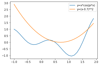
The excellent property of helping to span local minimum points or saddle points makes random gradient descent a more widely used optimization algorithm than gradient descent. Of course, to achieve this, the core point is that the loss function of local data is inconsistent with that of all data, and the local law is inconsistent with the global law. In other words, in essence, we use the difference of laws between different data to help parameter points escape the local minimum trap.

Summarize the above process: the essence of SGD calculation is to update parameters with the help of local laws (rather than overall laws), and the inconsistency of local laws can keep the moving direction of parameters flexible during the moving process, and therefore can escape the trap of local minimum points or saddle points, but the cost of inconsistent directions is that they can not converge to a stable point, To improve this problem, additional optimization means are needed.

Of course, small batch gradient descent also has this property. In the field of machine learning, we often use local law inconsistency to expand the performance of the algorithm, such as the random forest in the integrated algorithm.

• Oscillation iteration and loss function fluctuation

Of course, another influence of the uncertainty of the parameter iteration direction is that it is easy to cause the overall loss function to fluctuate in the convergence process. In fact, it is not difficult to understand that as long as the travel direction of the parameters is not consistent with the gradient decreasing direction of the loss function of all data, as long as the direction adjustment of the parameters occurs midway, it will lead to the oscillation of the calculation result of the loss function constructed from all data. For example, during the iteration of the above example, we can observe the change of the overall MSE

w = 1.5
MSE_l = [MSELoss(x, w, y)]
for j in range(20):
    for i in range(2):
        w = w_cal(x[i], w, y[i], lr_gd, lr = 0.02, itera_times = 1)
        MSE_l.append(MSELoss(x, w, y))
MSE_l
#[array([[0.25]]),
# array([[0.212]]),
# array([[0.1308992]]),
# array([[0.11062326]]),
# ...
# array([[0.0506296]]),
# array([[0.05000753]]),
# array([[0.05062882]])]
plt.plot(list(np.arange(41)), np.array(MSE_l).flatten())

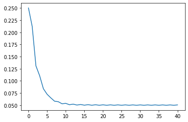
• Observe SGD iterative process with contour map

Of course, the fluctuation of the loss function in the above example is not obvious, but in the operation process of many complex models, the loss function will still be greatly affected by the inconsistent direction of each iteration. Of course, this influence can also be realized by observing the path in the process of parameter points approaching the global minimum point. For example, we conduct simple experiments with the help of the data and trajectory drawing function defined in Lesson 4.3.

np.random.seed(24)
w = np.random.randn(2, 1)                # All parameters are column vectors by default
w
#array([[ 1.32921217],
#       [-0.77003345]])
features = np.array([1, 3]).reshape(-1, 1)
features = np.concatenate((features, np.ones_like(features)), axis=1)
features
#array([[1, 1],
#       [3, 1]])
labels = np.array([2,4]),reshape(-1,1)
labels
#array([[2],
#       [4]])
# Random gradient descent parameter point trajectory
w_res = [np.copy(w)]
for i in range(40):
    w_res.append(np.copy(sgd_cal(features, w, labels, lr_gd, epoch=1, lr=0.1)))
w_res[-1]
#array([[1.00686032],
#       [0.96947505]])
np.random.seed(24)
w1 = np.random.randn(2, 1)                # All parameters are column vectors by default
w1
#array([[ 1.32921217],
#       [-0.77003345]])
# Gradient descent parameter point trajectory
w1, w_res_1 = w_cal_rec(features, w1, labels, gd_cal = lr_gd, lr = 0.1, itera_times = 100)
w_res_1[-1]
#array([[1.02052278],
#       [0.95045363]])
# Grid point coordinates
x1, x2 = np.meshgrid(np.arange(1, 2, 0.001), np.arange(-1, 1, 0.001))
# Draw contour map
plt.contour(x1, x2, (2-x1-x2)**2+(4-3*x1-x2)**2)

# Draw the trajectory diagram of parameter point movement
plt.plot(np.array(w_res)[:, 0], np.array(w_res)[:, 1], '-o', color='#ff7f0e', label='SGD')
plt.plot(np.array(w_res_1)[:, 0], np.array(w_res_1)[:, 1], '-o', color='#1f77b4', label='BGD')
plt.legend(loc = 1)

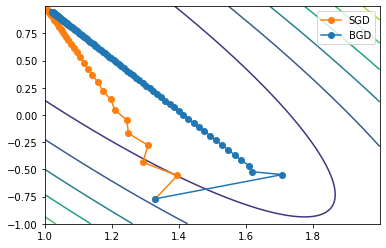
It can be seen that in the process of parameter iteration, the inconsistent direction of random gradient descent will have a great impact on the iterative process. As the saying goes, "those who succeed are destroyed". We use randomness to help the algorithm cross the local minimum trap, but it leads to other troubles - how to solve these "troubles" is the optimization algorithm around the random gradient descent algorithm that we will discuss later.

3. Solving linear regression by random gradient descent

Next, we try to use random gradient descent to solve the linear regression problem.

• Step 1. Identify data sets and models

The creation of disturbance items is still small and basically satisfied y = 2 x 1 − x 2 + 1 y=2x_1-x_2+1 y=2x1 − x2 + 1 regular data set.

# Set random number seed
np.random.seed(24)   

# The value of disturbance term is 0.01
features, labels = arrayGenReg(delta=0.01)

• Step 2. Set initial parameters

np.random.seed(24)  
w = np.random.randn(3, 1)
w
#array([[ 1.32921217],
#       [-0.77003345],
#       [-0.31628036]])
# SSE when calculating w value
SSELoss(features, w, labels)
#array([[2093.52940481]])
# MSE when calculating w value
MSELoss(features, w, labels)
#array([[2.0935294]])

• Step 3. Perform gradient descent calculation

Next, the gradient descent parameters are solved with the help of the previously defined parameter update function:

w = sgd_cal(features, w, labels, lr_gd, epoch=40, lr=0.02)
w
#array([[ 1.99749114],
#       [-0.99773197],
#       [ 0.99780476]])
# SSE when calculating w value
SSELoss(features, w, labels)
#array([[0.1048047]])
# MSE when calculating w value
MSELoss(features, w, labels)
#array([[0.0001048]])

So far, we have completed the complete process of solving the loss function by random gradient descent.

4. Evaluation of random gradient descent algorithm

According to the above discussion and implementation, we have basically mastered the basic idea and implementation method of solving the loss function by random gradient descent. Compared with gradient descent, random gradient descent introduces a certain randomness and jumps out of the local minimum point trap with the help of local law inconsistency, which can be said to be a major progress. In most complex models, the loss function is not necessarily a strictly convex function, so random gradient descent also has a wider application scenario than gradient descent.

However, it is worth mentioning that the calculation process of random gradient descent is still "too" random. In many complex models, the trouble of iterative convergence caused by this randomness is almost equal to the benefits brought by this randomness, such as more iterations and unstable final convergence results. It should be improved, One of the most basic methods we can think of is to increase the stability of some algorithms on the basis of ensuring a certain degree of randomness. That is, try to appropriately correct the sample size brought in by each iteration, that is, reasonably set the data volume brought in by the parameters of each iteration. On the one hand, we still hope to avoid the local minimum trap with the help of the uncertainty of the local law. At the same time, we also hope to control the randomness of the iterative process to a certain extent to reduce the trouble caused by randomness. This gradient descent algorithm, which brings several samples into each iteration process, is called small batch gradient descent.

Of course, if each data is basically consistent with the law of the overall data, such as (1,2), (2,4) data sets, the convergence efficiency of random gradient descent will be higher. After all, calculating a data is equivalent to calculating a data set. However, at this time, because there is no inconsistency of local laws between different data, random gradient descent can not help skip the local minimum point.

3, Mini batch gradient descent

The so-called small batch gradient descent is actually a slight modification of the random gradient descent process - not a piece of data is brought in each time for calculation, but a batch_size data for calculation, of course, batch_size is a manually set super parameter. Through such a small change, the actual performance of the algorithm will change fundamentally. At present, small batch gradient descent is also the most common algorithm in the gradient descent algorithm family.

For more performance comparison and algorithm optimization of gradient descent, random gradient descent and small batch gradient descent algorithms, see Lesson 4.4.

1. Small batch gradient descent calculation process

Similarly, we first observe the calculation process of gradient descent in small batch through a simple example. Take the opening dataset as an example:

When we perform small batch gradient descent, we will first segment the training data into "small batch". For example, we can segment the above data set into two mini batch. The first two data are the first batch and the last two data are the second batch. Then it is calculated according to the calculation process similar to random gradient descent.

• Data segmentation

x = np.array([1, 3, 6, 8]).reshape(-1, 1)
x
#array([[1],
#       [3],
#       [6],
#       [8]])
y = np.array([2, 5, 4, 3]).reshape(-1, 1)
y
#array([[2],
#       [5],
#       [4],
#       [3]])
x1 = x[:2]
x2 = x[2:4]
y1 = y[:2]
y2 = y[2:4]

• First round (epoch) iteration

After the data set segmentation is completed, we start to update the parameters. Like random gradient descent, when we traverse the data set once, it is called a round of epoch iteration completion. At this time, we divide the data set into two batches. After the two batches are brought into the training in turn, it is equivalent to the completion of the first round of epoch iteration.

w = 0
w = w_cal(x1, w, y1, lr_gd, lr = 0.02, itera_times = 1)
w = w_cal(x2, w, y2, lr_gd, lr = 0.02, itera_times = 1)
w
#array([[0.62]])

• Multi round (epoch) iteration

Of course, if you want to perform batch for more general data sets, you can manually adjust batch_size of small batch gradient descent calculation, we can put the above sgd_cal is modified to integrate small batch gradient descent and random gradient descent into one function. The specific calculation function is as follows:

def sgd_cal(X, w, y, gd_cal, epoch, batch_size=1, lr=0.02, shuffle=True, random_state=24):
    """
    Random gradient descent and small batch gradient descent calculation functions
    :param X: Training data characteristics
    :param w: Initial parameter value
    :param y: Training data tag
    :param gd_cal: Gradient calculation formula
    :param epoch: Number of traversal data sets
    :batch_size: Each small batch contains the number of data sets
    :param lr: Learning rate
    :shuffle: On each epoch Disorder the data set before starting
    :random_state: Random number seed value
    :return w: Final parameter calculation results       
    """
    m = X.shape[0]
    n = X.shape[1]
    batch_num = np.ceil(m / batch_size)
    X = np.copy(X)
    y = np.copy(y)
    for j in range(epoch):       
        if shuffle:                #Improve the generalization ability of the model
            np.random.seed(random_state)                           
            np.random.shuffle(X)                            
            np.random.seed(random_state)
            np.random.shuffle(y)    
        for i in range(np.int(batch_num)):
            w = w_cal(X[i*batch_size: np.min([(i+1)*batch_size, m])], 
                      w, 
                      y[i*batch_size: np.min([(i+1)*batch_size, m])], 
                      gd_cal=gd_cal, 
                      lr=lr, 
                      itera_times=1)
    return w

It should be noted here that the first is with the help of NP Ceil function calculation is divided into several batches. Note here that if the remaining data of the last batch is insufficient, batch_size quantity, you can also convert it into a batch. For example, taking x as an example, when every three pieces of data are divided into one batch, they can be divided into two batches in total

np.ceil(4 / 3)
#2.0

In addition, when performing the calculation, it is necessary to determine the upper bound of data set segmentation in the segmentation process

for i in range(2):                         # It is divided into two batches in total
    print(x[i*3: np.min([(i+1)*3, 4])])    # There are three pieces of data in each batch, and the total amount of data is 4
#[[1]
# [3]
# [6]]
#[[8]]

At the same time, it should be noted that in order to ensure the generalization ability of the model itself, generally speaking, we need to disorder the data set before each round of epoch. So far, we have completed the calculation function of gradient descent in small batch. We can simply check the calculation process:

# The initial parameter is 0, the two pieces of data are 1 batch, and the iteration is 1 round of epoch
w = 0
sgd_cal(x, w, y, lr_gd, epoch=1, batch_size=2, lr=0.02, shuffle=False)
#array([[0.62]])
# The initial parameter is 0, the two pieces of data are 1 batch, and the iteration is 10 rounds of epoch
w = 0
sgd_cal(x, w, y, lr_gd, epoch=10, batch_size=2, lr=0.02)
#array([[0.67407761]])
# The initial parameter is 0, the two pieces of data are 1 batch, and the iteration is 10 rounds of epoch
w = 0
sgd_cal(x, w, y, lr_gd, epoch=10, batch_size=2, lr=0.02)
#array([[0.52203531]])
# Contrast gradient descent calculation process
w = 0
w_cal(x, w, y, lr_gd, lr = 0.02, itera_times = 10)
#array([[0.56363636]])

Moreover, if the data volume of each batch of data is set to the total number of samples, the calculation process is equivalent to gradient descent

w = 0
sgd_cal(x, w, y, lr_gd, epoch=10, batch_size=4, lr=0.02)
#array([[0.56363636]])

Of course, if the data amount of each batch of data is set to 1, the calculation process is equivalent to random gradient descent

w = 0
for j in range(10):
    for i in range(4):
        w = w_cal(x[i], w, y[i], lr_gd, lr = 0.002, itera_times = 1)
w
#0.5347526106195503

w = 0
w = sgd_cal(x, w, y, lr_gd, epoch=10, batch_size=1, lr=0.002, shuffle=False)
w
#array([[0.53475261]])

2. Characteristics of small batch gradient descent algorithm

Although small batch gradient descent brings in more data for parameter training each time, its algorithm characteristics are similar to random gradient descent. In the training stage, each training actually uses the comprehensive law (comprehensive loss function) of a batch of data for parameter training. At the same time, Small batch gradient descent also helps the parameters jump out of the local minimum trap with the help of the law inconsistency of different batch data. Moreover, due to the law inconsistency, the final convergence result of small batch gradient descent will also show a small oscillation. However, in all aspects of "random uncertainty", small batch gradient descent is more robust than random gradient descent. Of course, when necessary, we will also convert small batch gradient descent into gradient descent or random gradient descent. More algorithm selection and optimization theories will be discussed in detail in the next section.

3. Small batch gradient descent to solve linear regression

Finally, we try to use small batch gradient descent to solve the linear regression problem. We will use a more formal process for calculation.

First of all, we still create a disturbance term that is small and basically satisfied y = 2 x 1 − x 2 + 1 y=2x_1-x_2+1 y=2x1 − x2 + 1 regular data set.

# Set random number seed
np.random.seed(24)   

# The value of disturbance term is 0.01
features, labels = arrayGenReg(delta=0.01)

Then perform data set segmentation

Xtrain, Xtest, ytrain, ytest = array_split(features, labels, rate=0.7, random_state=24)
Xtrain.shape
(700, 3)

Next, set the initial parameters

np.random.seed(24)  
w = np.random.randn(3, 1)
w
#array([[ 1.32921217],
#       [-0.77003345],
#       [-0.31628036]])

Then the parameters are solved by means of small batch gradient descent

w = sgd_cal(Xtarain, w, ytrain, lr_gd, batch_size=100, epoch=40, lr=0.02)
w
#array([[ 1.99975664],
#       [-0.99985539],
#       [ 0.99932797]])

Calculate training error and test error

# Training error
MSELoss(Xtrain, w, ytrain)
#array([[9.43517576e-05]])
# Test error
MSELoss(Xtest, w, ytest)
#array([[9.01449168e-05]])

For the algorithm to solve the numerical solution, observing its iterative process is the first step of subsequent optimization. Therefore, we can write the following process to observe how the model training error and test error change with the iteration.

np.random.seed(24)  
w = np.random.randn(3, 1)

trainLoss_l = []
testLoss_l = []

epoch = 20

for i in range(epoch):
    w = sgd_cal(Xtrain, w, ytrain, lr_gd, batch_size=100, epoch=1, lr=0.02)
    trainLoss_l.append(MSELoss(Xtrain, w, ytrain))
    testLoss_l.append(MSELoss(Xtest, w, ytest))
    
plt.plot(list(range(epoch)), np.array(trainLoss_l).flatten(), label='train_l')
plt.plot(list(range(epoch)), np.array(testLoss_l).flatten(), label='test_l')
plt.xlabel('epochs')
plt.ylabel('MSE')
plt.legend(loc = 1)