General classification:

Internal sorting

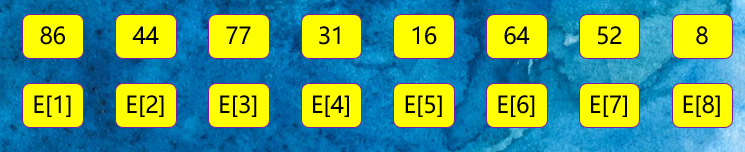
The amount of data is small, and all data can be sorted in memory. All sorting in this paper is from small to large

1. Insert sort

Insertion sort is one of the simplest sorting methods. In order to ensure the efficiency of random access, insertion sort should use array structure to complete random access to elements. Its overall idea is divided into three steps

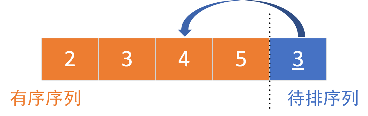
The execution of insert sort is illustrated below

Insertion sorting can include direct insertion sorting, half insertion and Hill sorting according to the methods of locating the insertion position. Here are three most commonly used insertion sorting methods:

1.1 direct insertion sort

1.1.1 direct insertion sorting principle

The simplest way to insert sorting is to insert sorting directly:
Direct insert sort refers to——
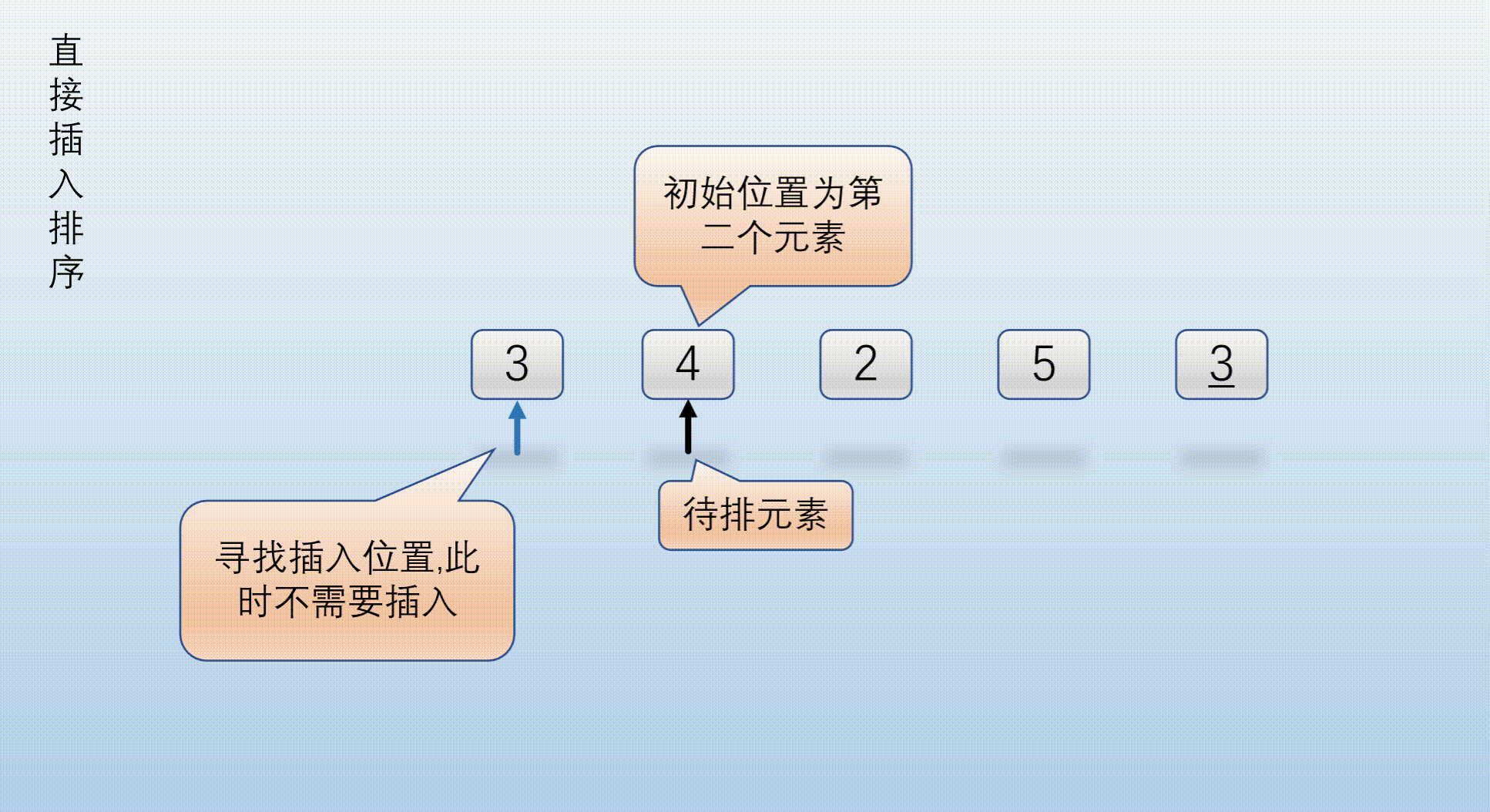
For an array of N elements starting from 0: N elements [0] ~ element [N-1] of a sequence, you can traverse the elements from 1 to N-1 (starting from the second element of the array), that is, N-1 times.

In the sorting process, "I" is used as the position mark of the current traversal Element. In a certain sorting, the first i-1 elements of sequence Element [] Element[0] ~ Element [i-1] have been ordered, while the range Element [i] ~ Element [n-1] has no order, In this sorting, find a position from the range Element[0] ~ Element [i-1] (mark the current position to be inserted with "j"), move Element [j] ~ Element [i-1] one bit back to Element [j + 1] ~ Element [i], and insert Element [I] into this position after moving Element back. At this time, the range Element[0] ~ Element [i] is in order.

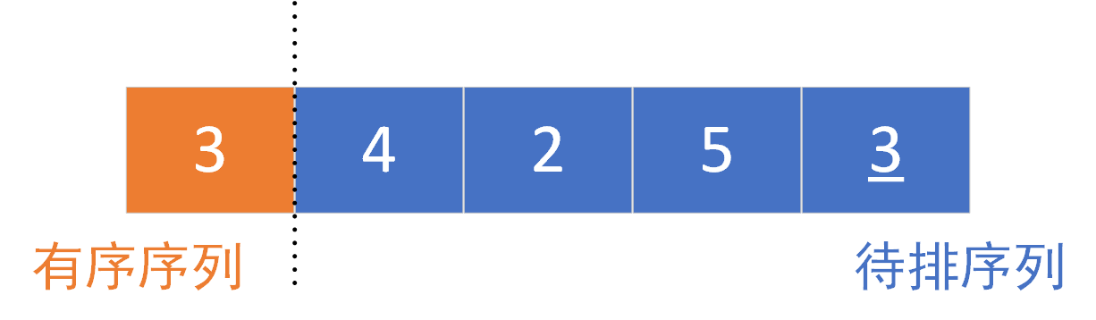
The specific execution diagram is as follows:
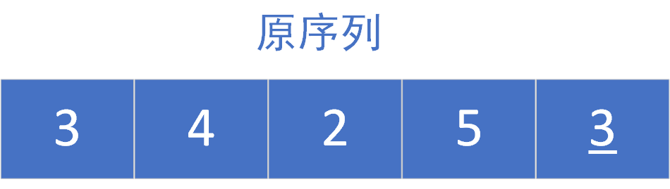
The original sequence is as follows:

First sorting:
The left part is the ordered part and the right part is the part to be sorted. It is sorted from the second element, 4 > 3 (element [1] > = element [0]). The original sequence is orderly and does not move the position

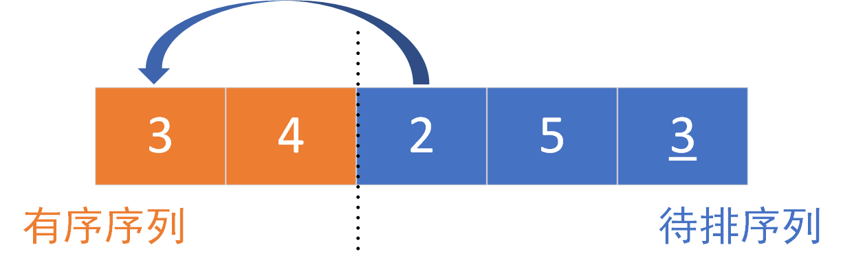
Second sorting:
The left part is the ordered part and the right part is the part to be sorted. Sort element [2], 2 > 3 (element [2] < element [0]). The insertion position is element [0], element [0] ~ element [1], move it one bit later and insert it

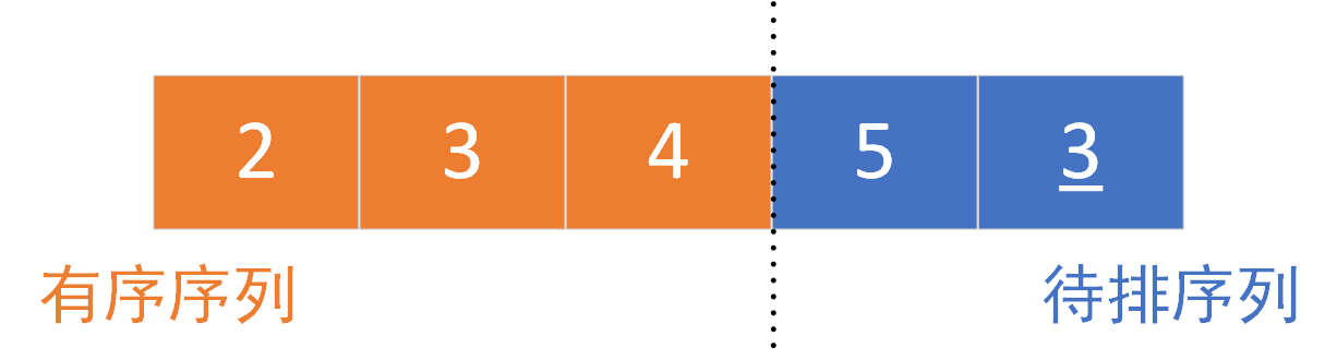
Third sorting:
The left part is the ordered part and the right part is the part to be sorted. Sort element [3], 5 > 4 (element [2] < element [3]). The original sequence is orderly and does not move the position

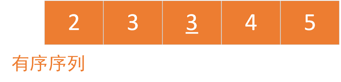
Fourth sorting:
The left part is the ordered part and the right part is the part to be sorted. Sort element [4], 4 > 3 (element [4] < element [2]). The insertion position is element [2]. Move element [2] ~ element [3] back one bit and then insert

After four sorting, the results are as follows:

1.1.2 direct insertion sort dynamic diagram

The sorting diagram uses the above example:

1.1.3 insert sort code directly

In this example, the C code for direct insertion sorting is given. Here are two writing methods. The first is the more traditional insertion sorting method. If temp is less than j, the element pointed to will be moved back.
The first writing method is as follows

//The first way of writing
void Insert_sort_inline(int Element[],int N) {
	int temp = 0;
	int j = 0;
	int i = 1;
	for (i = 1; i < N; i++){//The first For loop completes the traversal of N-1 elements
		temp = Element[i];
		j = i;
		while(j>0&&temp<Element[j-1]) {//In order to move the element position backward, scan from back to front. If temp is less than j, the element pointed to will be moved backward
			Element[j] = Element[j - 1];
			j--;
		}
		Element[j] = temp;
	}
}

The second way to write a direct insertion sorter is to make a special definition of an array, such as an array. The general definition is as follows:

int A[]={1,2,3,4,5}

Where A[0]=1,A[1]=2... And so on, when using an array, you can use the elements in an array as variables to simplify the boundary conditions, so as to prevent crossing the boundary when traversing the array. The variables of this array generally use the boundary elements in the array as intermediate variables, which can also be called sentinels.
For example, you can use the A[0] element as the sentinel of the array, that is, you can use A[0] as the boundary condition for finding the insertion position
Therefore, the second writing method is as follows

void Insert_sort_inline_with_sentry(int Element[], int N) {
	int i=0, j=0;
	for (i = 2; i <=N; i++) {
		Element[0] = Element[i];
		//Here you can use the For loop to complete the sorting
		//for (j = i - 1; Element[0] < Element[j]; j--)
			//Element[j + 1] = Element[j];
		j = i;
		while(Element[0]<Element[j-1]) {
			Element[j] = Element[j - 1];
			j--;
		}
		Element[j]=Element[0];
	}
}

Insertion sort needs to use the random access feature of the array, but it does not mean that the chain structure can not use insertion sort. The chain structure has multiple free pointers that can locate the absolute and relative positions of elements, or it can be an insertion sort.
Programming is flexible, but efficiency is unique.

1.1.4 complexity and stability of direct insertion sorting

Stability mainly considers whether to maintain the original order after sorting the same elements. In this example 3 3 3 and 3 ‾ \underline{3} 3. Keep the original order after sorting. So direct insertion sort is a stable sort.

1. Best case: the original sequence is ordered, and the complexity is O ( N ) O(N) O(N)
2. Worst case: the original sequence is in reverse order and the time complexity is O ( N 2 ) O(N^{2}) O(N2)
3. Average time complexity: O ( N 2 ) O(N^{2}) O(N2)
4. Space complexity is constant: O ( 1 ) O(1) O(1)

1.2 split insertion sort

In the process of finding the insertion position, the half search method is used to find the insertion position. This insertion method is called half insertion sorting.
All elements before the "i" of the insertion sort are ordered, so it is convenient to use half search to find the insertion position. Here is a brief introduction to half search:

1.2.1 half search

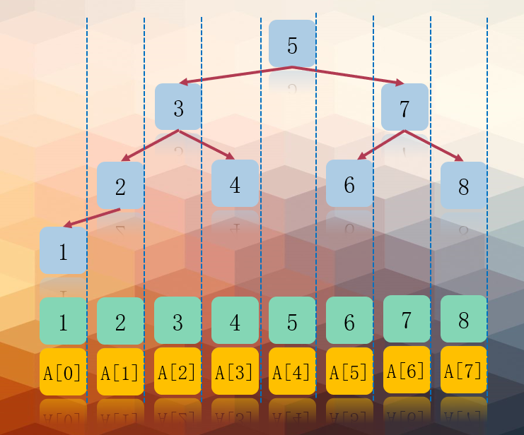
In fact, half search is to use binary tree sorting tree to complete the search operation. Here is a binary sorting tree structure for readers' reference. The characteristics of binary sort tree are as follows:
1. If the left subtree is not empty, the values of all nodes on the left subtree are less than the values of its root node;
2. If the right subtree is not empty, the values of all nodes on the right subtree are greater than the values of its root node;
3. The left and right subtrees are also binary sort trees respectively;
4. There are no nodes with equal values.

For the ordered queue, the following sort tree can be generated. The search of the sort tree is not the focus of this paper. Later, the author will update the summary of the search algorithm. The node Element[mid] searched by the binary sort tree is the root node of the sort tree. If the searched value is greater than the root node, it will turn to the right subtree, and if the value is less than the root node, it will turn to the left subtree.

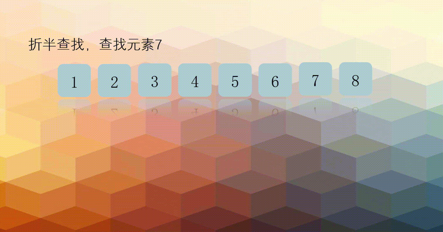
1.2.2 half search diagram

Taking the sequence element [] = {1,2,3,4,5,6,7,8} as an example, the execution diagram of finding 7 is as follows:

1.2.3 half search code

The half search code is as follows:

//x represents the element to be found
int Half_fold_search(int Element[], int low, int heigh,int x) {
	
	while (low<=heigh)
	{
		int mid = (low + heigh) / 2;//Define intermediate variables
		if (Element[mid] == x)//If the element location is found, the location is returned
			return mid;
		else if (x > Element[mid])
			low = mid + 1;
		else
			heigh = mid - 1;
		
	}
	return -1;//Low > height, return - 1, indicating that there is no element to look for in the sequence
}

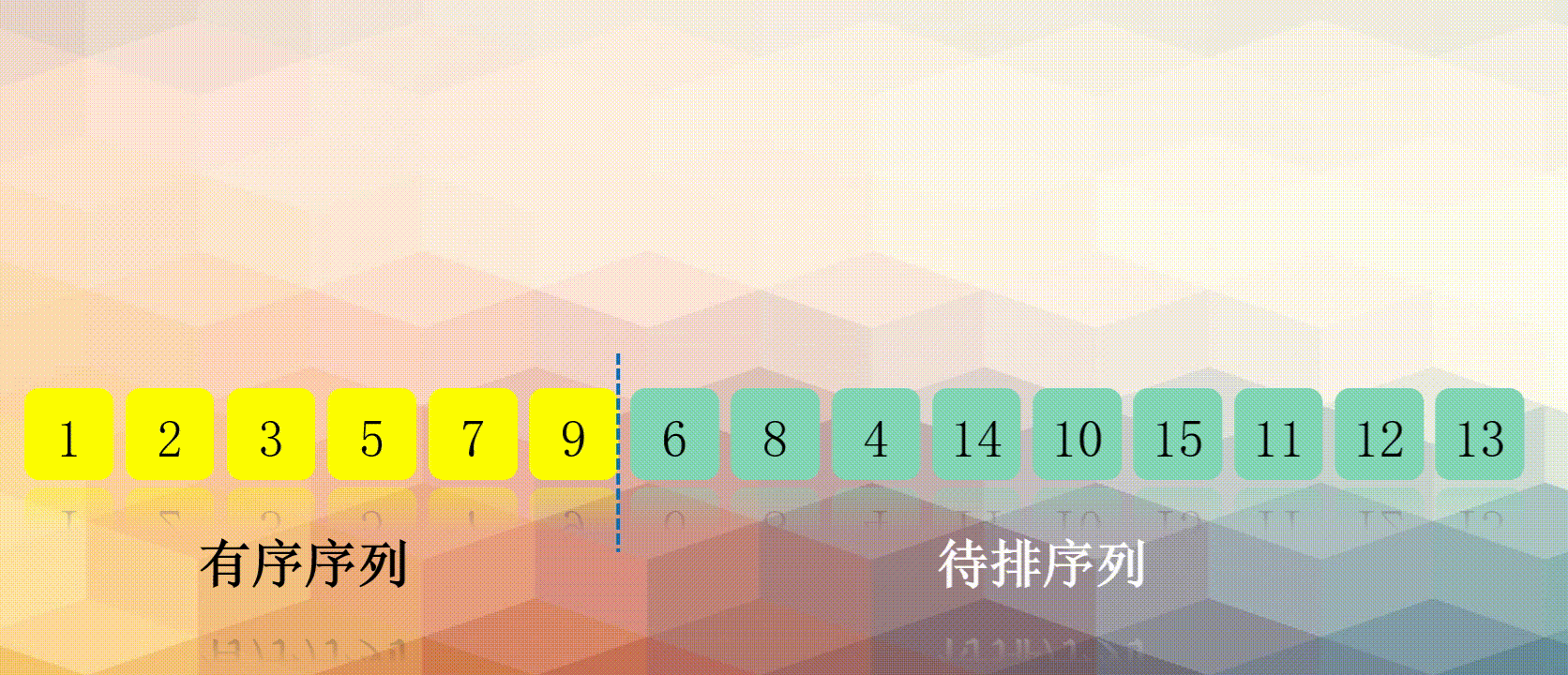
1.2.4 split insertion sorting diagram

In this example, the result after the half search position is given l o w low low and h e i g h heigh The position when the heigh t two markers find the insertion position is as follows. The insertion position can be l o w low low and h e i g h + 1 heigh+1 heigh+1:

1.2.5 insert sort code in half

In this paper, the code of half insertion sorting using sentinel is given. Readers can simply modify it according to the actual application:

//Binary Insertion Sort 
void Half_fold_Insert_sort(int Element[],int N) {
	int i = 0, j = 0, mid = 0, low = 0, heigh = 0;
	for (i = 2; i <N;i++) {
		//Half find insertion position
		Element[0] = Element[i];
		low = 1;
		heigh = i - 1;
		while (low<=heigh)
		{
			mid = (low + heigh) / 2;
			if (Element[mid] > Element[0])
				heigh = mid - 1;
			else
				low = mid + 1;
		}
		//Move the element back when the insertion position is found
		for (j = i - 1; j >= heigh+1; j--)
			Element[j + 1] = Element[j];
		//Insert element where found
		Element[heigh + 1] = Element[0];
	}
}

1.2.6 sorting complexity and stability of half insertion

Half insertion sorting is a stable sorting method.

The half search only optimizes the number of comparisons, which is of the order of magnitude O ( N log ⁡ 2 N ) O(N\log_2N) O(Nlog2 ＾ N). Since N will affect the tree height of the binary sort tree, the comparison times of half search have nothing to do with whether the initial sort is ordered, but only with the number of sequence elements. However, the optimization comparison times still need to move back elements, so the time complexity is O ( N 2 ) O(N^2) O(N2)

1. Average time complexity: O ( N 2 ) O(N^2) O(N2)
2. Space complexity is constant: O ( 1 ) O(1) O(1)

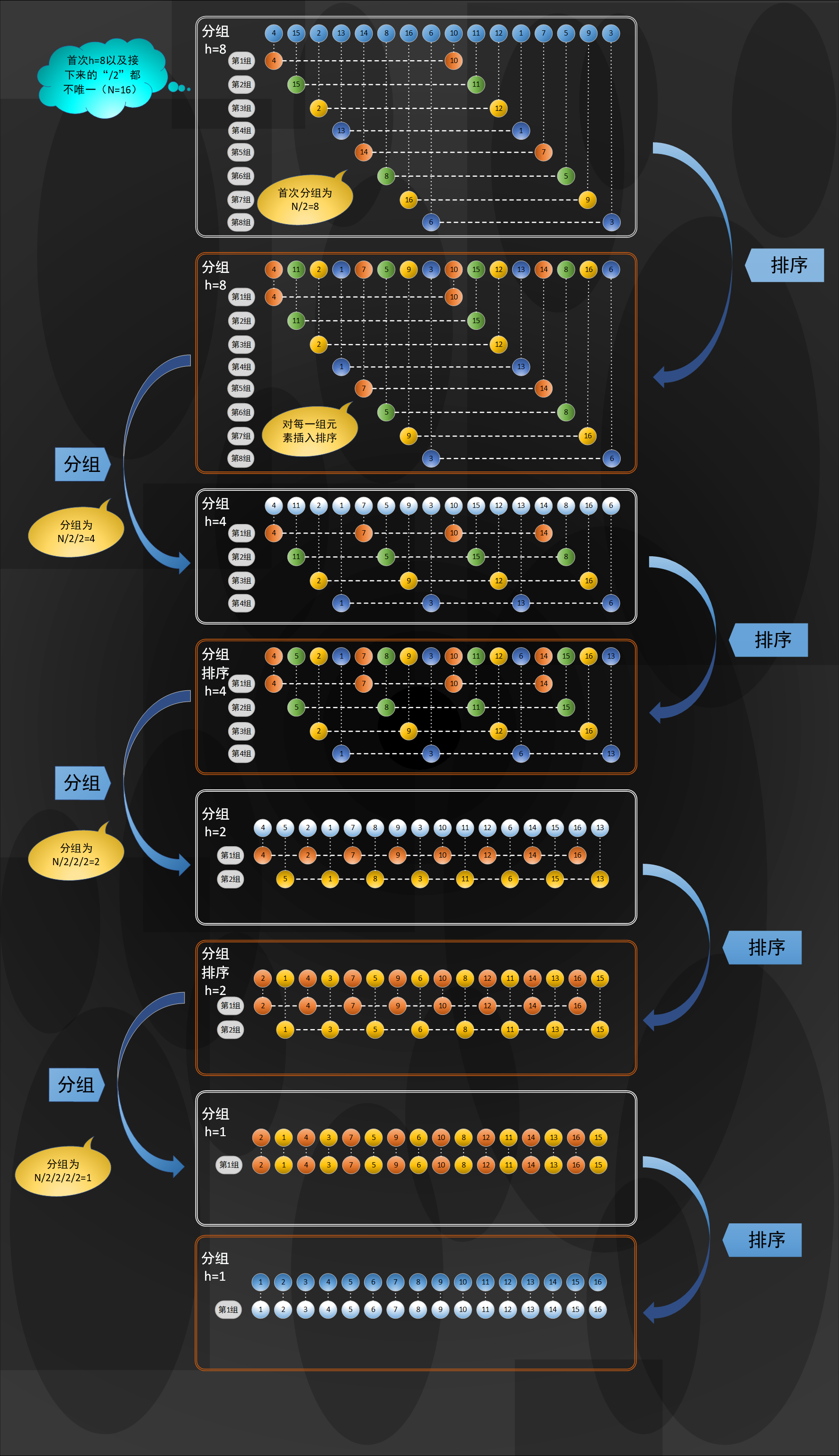
1.3 Hill sorting

Hill sorting is a sort algorithm proposed by Donald Shell in 1959. Hill sort is also an insertion sort. It is a more efficient version of simple insertion sort after improvement, also known as reduced incremental sort. At the same time, the algorithm breaks through N 2 N^{2} N2 is one of the first algorithms.
Hill's idea of sorting is actually a method of grouping insertion

The goal of Hill sort is to order the elements at any interval h in the middle of the array. The elements every H form an ordered array of H. An H ordered array is an array composed of H ordered subsequences
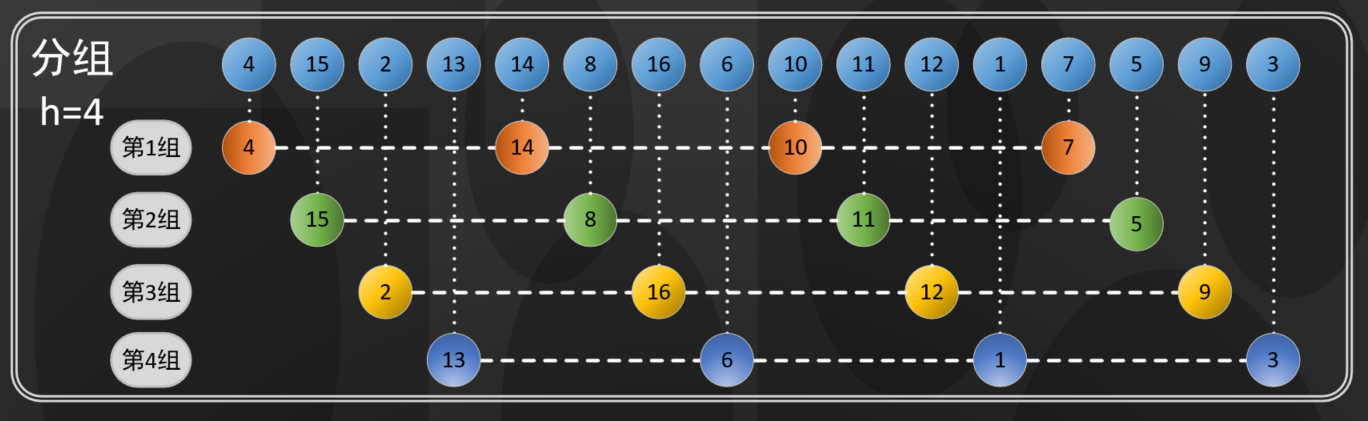
For example:
An array with a length of 16, as shown in the following figure when h=4:
In the figure above, every four elements are grouped, and each group is composed of four elements, a 4-ordered array

An array with a length of 16, as shown in the following figure when h=5:

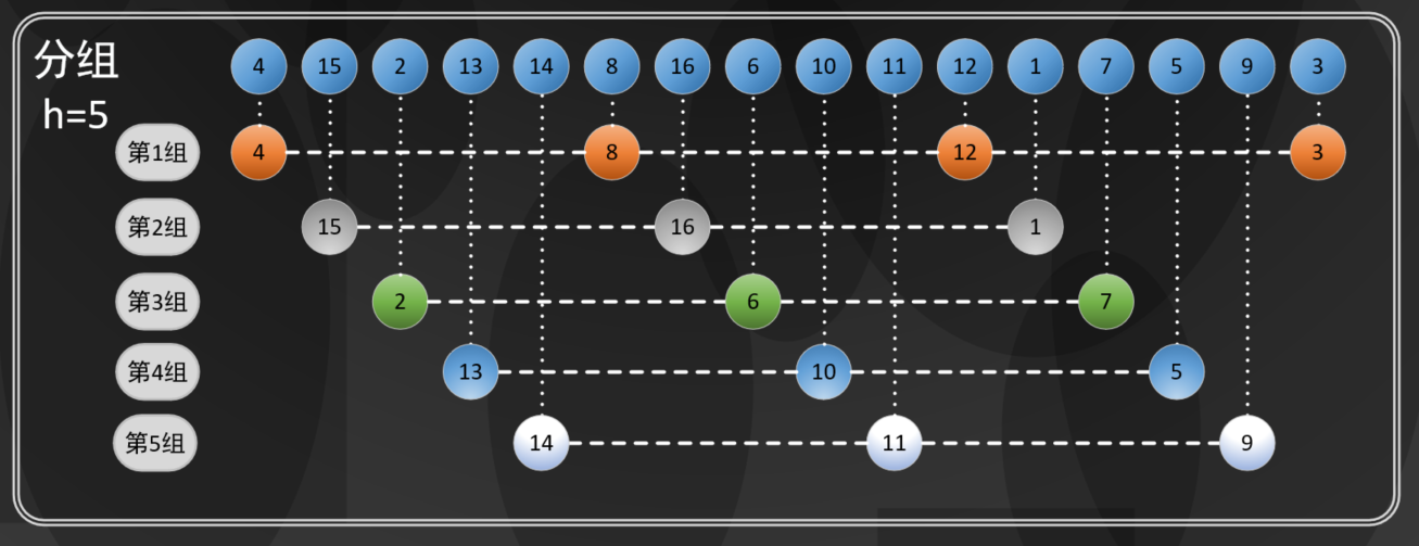
In the figure above, every five elements are grouped into a 5-ordered array

1.3.1 Hill ranking diagram

In order to facilitate readers' understanding, the following diagram of hill sorting is given as follows (you can click to zoom in):

The code is as follows,

void Shell_Sort(int Element[],int N) {
	int step = 0,i = 0,temp=0,j=0;
	for (step = N / 2; step >= 1;step/=2) {//Adjust the step length by 2
		for (i = step; i < N; i++) {
			if (Element[i] < Element[i - step]) {//Compare each set of elements
				temp = Element[i];
				for (j = i - step; j >= 0 && temp < Element[j]; j -= step)//Move back element
					Element[j + step] = Element[j];
				Element[j + step] = temp;
			}
		}
	}
}

1.3.2 complexity and stability of Hill ranking

Stability:
Hill sorting will group the sequences according to a fixed length step, so the relative position of the original sequence cannot be guaranteed for the elements with the same value. Hill sorting is an unstable sorting algorithm.
Time complexity:
The complexity of hill sorting is related to the increasing sequence. The performance of the algorithm depends not only on h, but also on the mathematical properties between h, such as grouping (4, 2, 1) or grouping (9, 3, 1). Therefore, it is difficult to describe its sorting method for the performance characteristics of out of order arrays. Different incremental sequences have different time complexity.

• {1,2,4,8,...} this sequence is not a good incremental sequence. The time complexity (worst case) of using this incremental sequence is N 2 N^{2} N2
• Hibbard proposed another incremental sequence {1,3,7, 2 k − 1 2^{k}-1 2k − 1}, the time complexity (worst case) of this sequence is N 3 / 2 N^{3/2} N3/2
• Sedgewick proposed several incremental sequences, and the worst-case running time is N 1.3 N^{1.3} N1.3. The best sequence is {1,5,19,41109,...}

Hill sort still has good performance for medium-sized arrays, with small amount of code and no additional space. It is a good choice when extreme operating environment is not required.

2. Exchange sorting

The idea of exchange sort is to select two elements each time for comparison and exchange positions. The most common exchange sort is bubble sort and quick sort.

2.1 bubble sorting

Bubble sort is a very vivid exchange sort method. The sequence is sorted in a bubble way, and every two elements are exchanged from bottom to top.

2.1.1 bubble sorting diagram

This sort of exchange is believed to be understood by readers according to the diagram, which is as follows:

2.1.2 bubble sort code

///Bubble sorting
void Bubbling_Sort(int Element[],int N) {
	int temp = 0;
	for (int i = 0; i < N - 1; i++) {
		bool flag = false;//Set the exchange flag bit. If true, it indicates that exchange has occurred
		for (int j = N - 1; j > i;j--) {
			//Sort from back to front to find the smallest element first
			if (Element[j-1]>Element[j]) {//Exchange occurs when the current element is greater than the previous element
				temp = Element[j - 1];
				Element[j - 1] = Element[j];
				Element[j] = temp;
				flag = true;//Modify the flag bit to indicate that an exchange has occurred
			}
			
		}
		if (flag == false)//The sequence is already ordered and does not need to be sorted
			return;
	}
}

2.1.3 complexity and stability of bubble sorting

1. Average time complexity: O ( N 2 ) O(N^{2}) O(N2)
2. Space complexity is constant: O ( 1 ) O(1) O(1)

Bubble sorting has good adaptability to linked lists and does not depend on the random access of arrays. It is a stable sorting method.

2.2 quick sort

When readers understand quick sorting, they can first try to read the merging sorting of this article, which is helpful to understand the idea of partition and rule

In fact, the quick sort process is also a sort algorithm of divide and conquer. Quick sort and merge sort are complementary. Merge sort divides the array into two sub arrays, sorts them respectively, and merges the ordered sub arrays in a recursive way to get the whole ordered array.
Therefore, the main steps of the sorting algorithm are:

1. First, take a number from the sequence as the reference number.
2. In the partition process, all numbers larger than this number are placed on its right, and all numbers less than or equal to it are placed on its left.
3. Repeat the second step for the left and right intervals until there is only one number in each interval.

In general, quick sort still uses the idea of exchange. As shown in the figure below, set two "pointers" to traverse the sequence from both sides, and find the elements with the left half greater than 6 and the right half less than 6 for exchange.

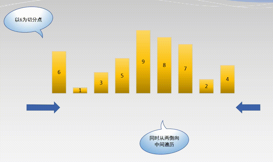
2.2.1 quick sort diagram

2.2.2 quick sort code

///< quick sort >
///< / group sort process >
int Partition(int Element[],int low,int heigh) {
	int Current_Element = Element[low];//Select flag element
	while (low<heigh)
	{
		while (low < heigh && Element[heigh] >= Current_Element)
			--heigh;//The element is smaller than the flag element and moves to the left
			Element[low] = Element[heigh];
		while (low < heigh && Element[low] <= Current_Element)
			++low;//Element larger than the flag element moves to the right
			Element[heigh] = Element[low];
	}
	Element[low] = Current_Element;
	return low;
}
///< quick sort >
///< / sort process >
void Quick_Sort(int Element[], int low, int heigh) {
	if (low < heigh) {
		int Current_Element = Partition(Element, low, heigh);
		//Right and left parts
		Quick_Sort(Element,low, Current_Element-1);
		Quick_Sort(Element, Current_Element+1,heigh);
	}
}

2.2.3 complexity and stability of quick sort

Quick sort is an unstable sort method. Similar to the split search insertion sort, quick sort is actually an application for red black trees.
The average time complexity is: O ( N log ⁡ 2 N ) O(N\log_2N) O(Nlog2​N)
The average space complexity is: O ( log ⁡ 2 N ) O(\log_2N) O(log2​N)
The application of quick sort is not strong for partially ordered sequences. If the sequences are ordered, the time complexity is about O ( N 2 ) O(N^2) O(N2)

3 select sort

The idea of selective sorting is to select the smallest element from the to be arranged sequence and store it in the existing sequence until there is only one element in the to be arranged sequence.

3.1 simple selection sorting

The implementation process of simple selection sorting is relatively simple. The code is given directly in this paper and will not be explained in detail.

3.1.1 simple selection of sorting code

void Simple_Select_Sort(int Element[], int N) {
	//Simple selection sort
	int min = 0;
	int temp = 0;
	for (int i = 0; i < N; i++) {//Traverse all elements in the sequence
		min = i;
		for (int j = i + 1; j < N; j++)//Find the minimum value between the current element and the last element
			if (Element[j] < Element[min])
				min = j;
		if (min != i) {//exchange
			temp = Element[i];
			Element[i] = Element[min];
			Element[min] = temp;
		}
	}
}

3.1.2 complexity and stability of simple selection sorting

Simple selection sorting is an unstable sorting method. This is because only a single element is selected to complete the sorting process at a time.
Space complexity: O ( 1 ) O(1) O(1)
Time complexity: O ( N 2 ) O(N^2) O(N2)

3.2 heap sorting

The optimization of selection sort is the optimization of selection method and selection process. Heap sort is an excellent way to simplify selection.

3.2.1 execution diagram of heap sorting

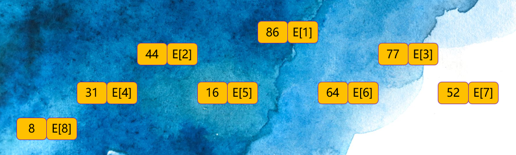
Heap sorting consists of heap building and sorting. The example sequence is as follows:

The first reactor building process is as follows:
The binary tree is established according to the position between the elements represented by the array

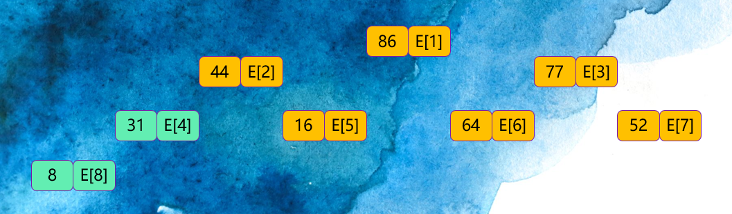
from E [ ⌊ N / 2 ⌋ ] E[\lfloor N/2 \rfloor] Start to complete the adjustment at E [⌊ N/2 ⌋], and check it first E [ ⌊ N / 2 ⌋ ] E[\lfloor N/2 \rfloor] Whether there are left and right nodes at E [⌊ N/2 ⌋]. If so, find out the maximum value of the left and right nodes and compare it with this node. Find the maximum value and replace it with the current value. In this example, from E [ 4 ] E[4] Start adjustment at E[4]:
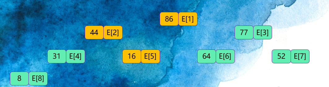
stay E [ 4 ] E[4] Traverse after adjustment at E[4] E [ 3 ] E[3] For node E[3], the maximum value of the two child nodes is 64 and less than 77, so no adjustment is made

stay E [ 3 ] E[3] Traverse after adjustment at E[3] E [ 2 ] E[2] For node E[2], the maximum value of the two child nodes is 31 less than 44, so no adjustment is made, E [ 1 ] E[1] The same operation is performed at E[1], so the large root heap is as follows:

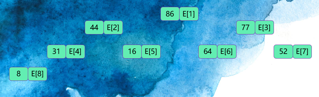
The overall sorting method is as follows:

3.2.2 execution code of heap sorting

//Perform root heap adjustment and establish
void Root_Pile(int Element[], int k, int N) {
	 Element[0] = Element[k];
	 for (int i = 2 * k; i < N; i *= 2) {
		 if (i < N && Element[i] < Element[i + 1])
			 i++;
		 if (Element[0] >= Element[i])
			 break;
		 else {
			 Element[k] = Element[i];
			 k = i;
		 }
	}
	 Element[k]=Element[0];
}
///Build large root heap
void Buid_Large_Root_Pile(int ELement[],int N) {
	for (int i = N / 2; i >= 0; i--)
		Root_Pile(ELement,i,N);
}
//Heap sorting process
void Heap_Sort(int ELement[], int N) {
	int temp = 0;
	Buid_Large_Root_Pile(ELement,N);
	for (int i = N; i > 1; i--) {
		temp = ELement[i];
		ELement[i] = ELement[1];
		ELement[1] = temp;
		Root_Pile(ELement,1,i-1);
	}
}

3.2.3 complexity and stability of heap sequencing

Heap sort is an unstable sort method.
The space complexity is: O ( 1 ) O(1) O(1)
The time complexity is: O ( N log ⁡ 2 N ) O(N\log_2 N) O(Nlog2​N)

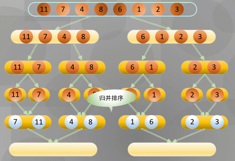
4 merge sort

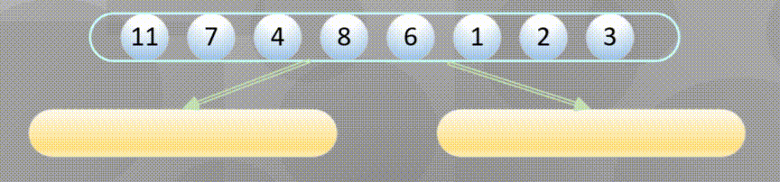
Merging adopts a divide and conquer idea, which regards a sequence as a combination of many small sequences. The process of merging is to merge the current ordered sequences.
For example, in terms of two-way merging, it is to merge two ordered tables into an ordered table to obtain a complete ordered sequence.
Merging is an idea of sacrificing space to steal time efficiency

The characteristics of merging and sorting are as follows. Readers can understand the following two points according to the diagram and code:

• Merge sort can ensure that any length is N N The time and cost required to sort an array of N N log ⁡ 2 N N\log_2N Nlog2 is proportional to N;
• The main disadvantage of merge sorting is the additional space and N N N is proportional.
  Note: the merging introduced in this paper is mainly two-way merging, and multi-way merging is widely used in external sorting. This paper does not involve external sorting.

4.1 in situ merging and sorting method

Here is the most common way to merge and sort - one way to merge is to directly merge two ordered arrays into another array. The diagram is as follows:

1. First, sort the left and right sequences a [ k ] a[k] a[k] copy all elements to a u x [ k ] aux[k] In aux[k]:

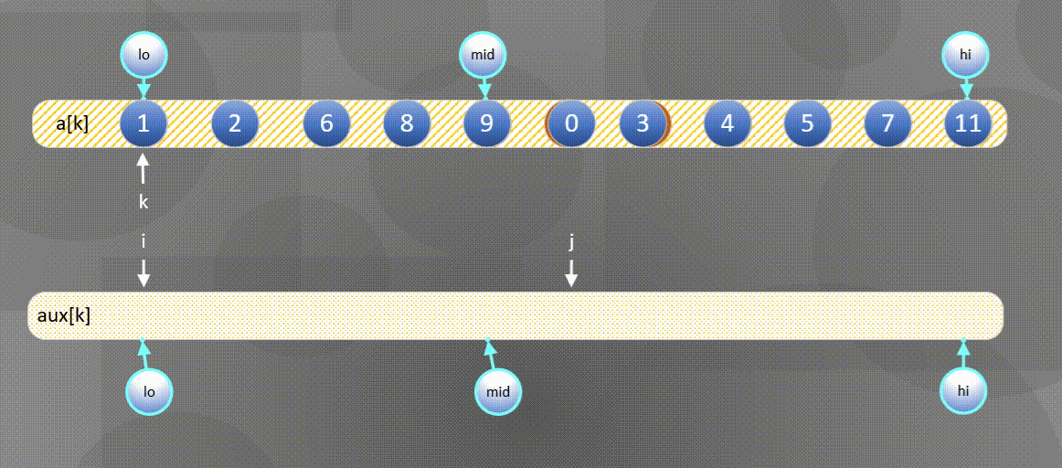
2. Then a u x [ k ] aux[k] Merge elements in aux[k] into a [ k ] a[k] a[k].

• If the right element is small, the a u x [ j ] aux[j] Merge elements in aux[j] into a [ k ] a[k] In a[k],
• If the left element is small, the a u x [ i ] aux[i] Merge elements in aux[i] into a [ k ] a[k] a[k].
  
  
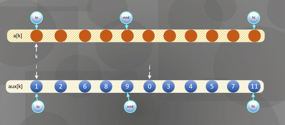
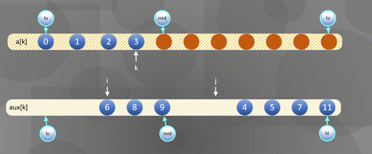
  The left side is exhausted and the second half is directly a u x [ j ] aux[j] aux[j] copy to a [ k ] a[k] a[k]

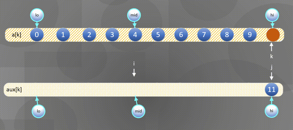
In situ merging algorithm is as follows:

void Merge(int Element[],int Element_Copy[], int low, int mid, int heigh) {//Complete the merging process of the two sequences
	//Complete the replication of the two sequences
	for (int h = low; h <= heigh; h++)
		Element_Copy[h] = Element[h];
	int i = low, j = mid + 1,k=low;
	for (int k = low; i < mid + 1 && j <= heigh; k++) {
	//Compare the size of the two parts of the sequence, and copy the small elements back to the original sequence
		if (Element_Copy[i] <= Element_Copy[j])
			Element[k] = Element_Copy[i++];
		else
			Element[k] = Element_Copy[j++];
	}
	while (i <= mid)
		Element[k++] = Element_Copy[i++];
	while (j <= heigh)
		Element[k++] = Element_Copy[j++];
}

Recursive sorting can be completed by calling the in place sorting process.

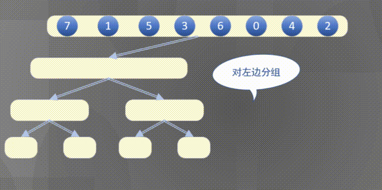
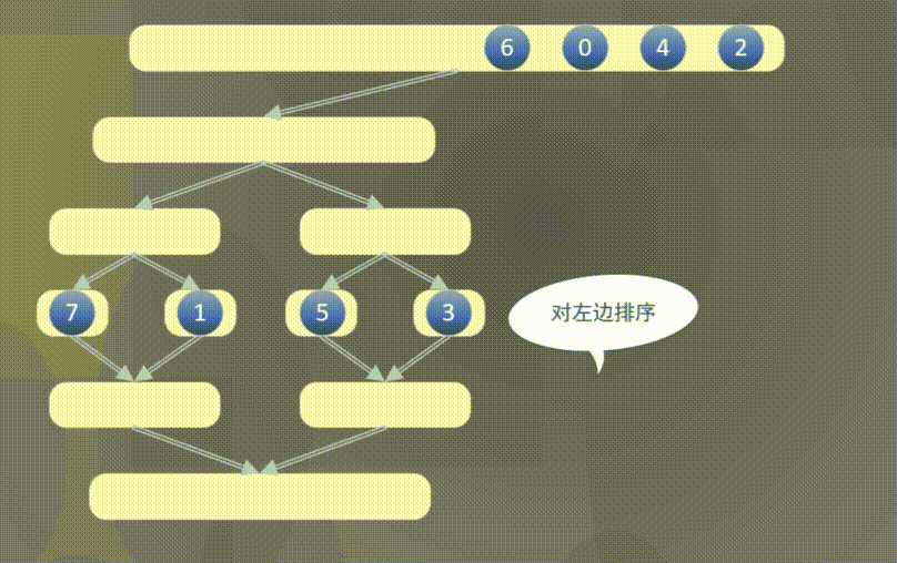
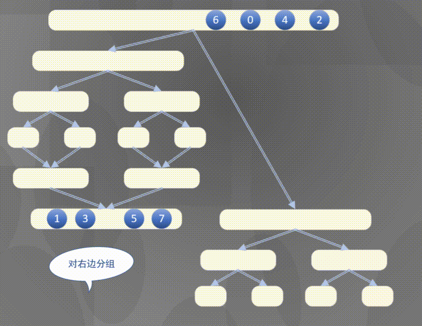
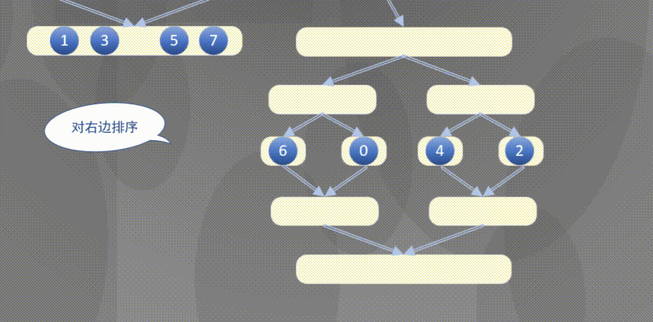
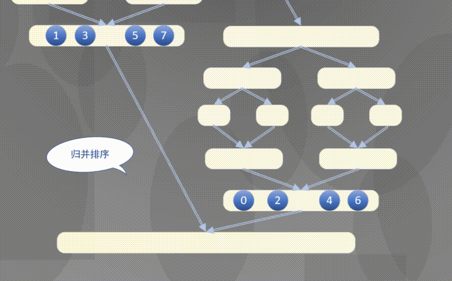
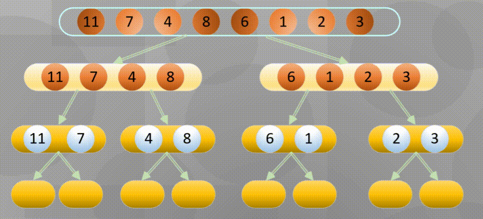
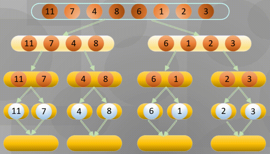
4.2 top down merge sort

4.2.1 top down merging and sorting diagram

Top down actually completes the sorting rules of the left array first and then the right array:

4.2.2 top down merge sort code

void Merge_Sort_Top_Down(int Element[], int Element_Copy[], int low, int heigh) {
	//Top down merge sort
	if (low < heigh) {
		int mid = (low + heigh) / 2;
		Merge_Sort_Top_Down(Element,Element_Copy,low,mid );//Merge and sort the left sequence first
		Merge_Sort_Top_Down(Element, Element_Copy, mid + 1, heigh);//Merge and sort the elements on the right
		Merge(Element,Element_Copy,low,mid,heigh);//Merge operation
	}
}

Actually, Merge_Sort is only used to complete reasonable calls in the order of merge execution.

It is directly given here that for the length N N N array, number of comparisons for top-down merge sort: 1 / 2 N l g N 1/2NlgN 1/2NlgN~ N l g N NlgN NlgN
Number of accesses to the array (maximum): 6 N l g N 6NlgN 6NlgN

4.3 bottom up merge sort

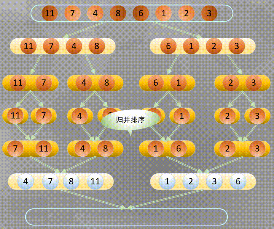
4.3.1 bottom up merging and sorting diagram

Bottom up is actually merging and sorting from the smallest group in all arrays
Decompose first, that is, the recursive process decomposes first and then sorts: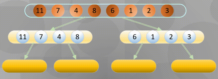

Merge in place when decomposing to the simplest element:

4.3.2 bottom up merge sort code

Readers can further understand the merging operation according to the code of bottom-up merging and sorting. The core of bottom-up merging and sorting is the grouping of sequences:

void Merge_Sort_Down_Top(int Element[], int Element_Copy[], int N) {
	int heigh_min=0;
	for (int sz = 1; sz < N; sz = sz + sz) {//Sets the length of the merged substring
		for (int lo = 0; lo < N - sz; lo += sz + sz)//Sets the starting position of the substring
		{	//The if statement is equivalent to min(N-1,lo+sz+sz-1), and the maximum length of the substring cannot exceed N-1
			if ((N - 1) > (lo + sz + sz - 1))
				heigh_min = lo + sz + sz - 1;
			else
				heigh_min = N - 1;
			Merge(Element, Element_Copy, lo, lo + sz - 1, heigh_min);
		}
	}
}

It is directly given here that for the length N N N array, number of comparisons for top-down merge sort: 1 / 2 N l g N 1/2NlgN 1/2NlgN~ N l g N NlgN NlgN
Number of accesses to the array (maximum): 6 N l g N 6NlgN 6NlgN

4.4 complexity and stability of merging and sorting

Merge operation will not change the relative order of the same keywords, so merge sorting is a stable sorting method.
Spatial replication: O ( N ) O(N) O(N)
Time complexity: O ( N log ⁡ 2 N ) O(N\log_2N) O(Nlog2​N)
The time complexity is mainly composed of two parts. The time complexity of merging operation is O ( N ) O(N) O(N), the operation of two-way merging is affected by the height of the merging tree, and the order of magnitude is O ( log ⁡ 2 N ) O(\log_2N) O(log2​N)

5 cardinality sorting

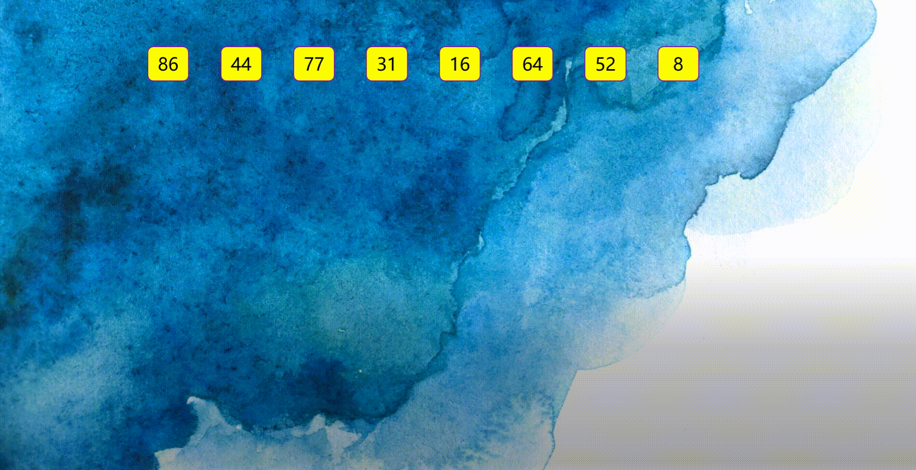
5.1 cardinality sorting diagram

Radix sorting is a non comparative integer sorting algorithm. Its principle is to cut integers into different numbers according to the number of bits, and then compare them according to each number of bits. The principle is to cut the sequence into different bits according to the number of bits (or other ways), and then compare them respectively according to each bit. In general, cardinality sorting can be divided into two categories:

1. MSD: sort from the high order first,
2. LSD: sort from the low order first,
   Examples of execution are as follows:
   

5.2 cardinality sorting code

int Max_Bit(int Element[], int N) //Find the maximum number of bits of data
{
	int maxData = Element[0];      
	///First find the maximum number, and then find the number of digits
	for (int i = 1; i < N; ++i)
	{
		if (maxData < Element[i])
			maxData = Element[i];
	}
	int d = 1;
	int p = 10;
	while (maxData >= p)
	{
		//p *= 10; // Maybe overflow
		maxData /= 10;
		++d;
	}
	return d;

//Cardinality sort
void Radix_Sort(int Element[], int N)
{
	int d = Max_Bit(Element, N);
	int* tmp = new int[N];
	int* count = new int[10]; //count
	int i, j, k;
	int radix = 1;
	for (i = 1; i <= d; i++) //Sort d times
	{
		for (j = 0; j < 10; j++)
			count[j] = 0; //Clear the counter before each allocation
		for (j = 0; j < N; j++)
		{
			k = (Element[j] / radix) % 10; //Count the quantity in each record
			count[k]++;
		}
		for (j = 1; j < 10; j++)
			count[j] = count[j - 1] + count[j]; //The positions in the tmp are assigned to each sequence in turn
		for (j = N - 1; j >= 0; j--) //Collect all records into tmp in turn
		{
			k = (Element[j] / radix) % 10;
			tmp[count[k] - 1] = Element[j];
			count[k]--;
		}
		for (j = 0; j < N; j++) //Copy the contents of the temporary array into the sequence
			Element[j] = tmp[j];
		radix = radix * 10;
	}
	delete[]tmp;
	delete[]count;
}

5.3 complexity and stability of merging and sorting

Cardinal sort is a sort method for specific data format. It can sort sequences without comparing elements. It is a special comparison algorithm. It is a stable sorting algorithm.

• Space complexity: O ( R ) O(R) O(R)
• Cardinality sorting requires D-pass allocation and collection, and one pass allocation requires O(N); O required for one trip collection ®， Therefore, the time complexity of cardinality sorting is O ( D ( N + R ) ) O(D(N+R)) O(D(N+R))

6 Summary of various sorting algorithms

The space and time complexity is summarized as follows (click to zoom in):

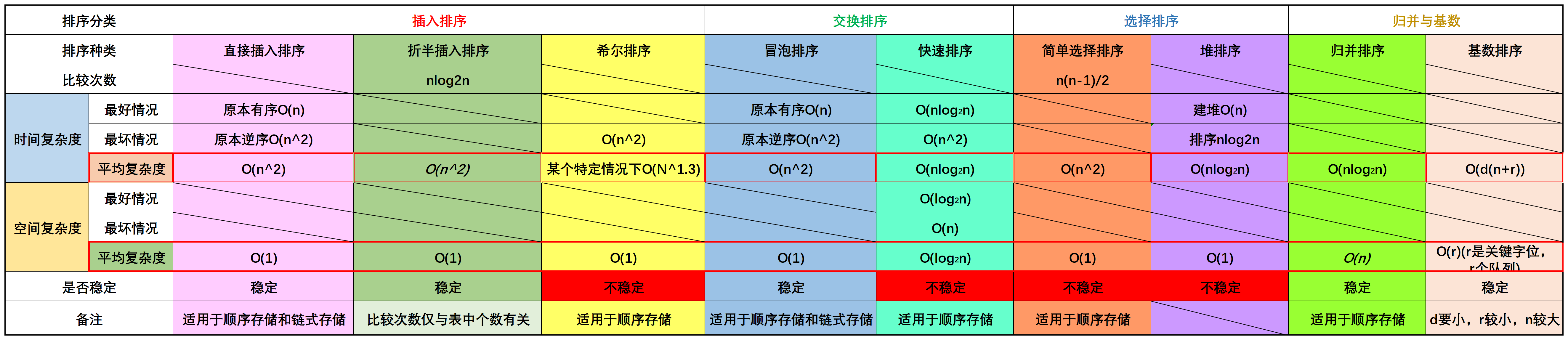
For the sorting algorithm, quick sort is the best in theory. Quick sort is a sort method using the idea of red black tree. The code is simple. It is a common and highly efficient sorting algorithm.
For heap sorting, although the space complexity is low, the root heap will be adjusted every time, and a lot of useless work has been done in the implementation of the algorithm.