Catalogue of series articles

Flink user's Guide: teach you to develop Flink SQL custom Connector, which is more convenient to use SQL for warehousing!

Flink user's Guide: Flink sets global variables and gets them in functions to make your code more elegant!

Flink user's Guide: the Checkpoint mechanism is completely understood. You are the boss!

Flink user's Guide: you must ask about the memory management model during the interview. You must know it when you enter a large factory!

Flink user's Guide: Kafka flow table associated with HBase dimension table

Flink user's Guide: using the new version of Watermark

Flink user's Guide: Flink SQL custom functions

catalogue

preface

MiniBatch aggregation

Local global aggregation

Split distinct aggregation

Use the FILTER modifier on a distinct aggregate

preface

Old rules, daily map, goddess town building map

We all know that the concept of Flink multi flow Join is mainly divided into bounded flow Join and unbounded flow Join

The main implementation method of bounded flow Join is to open a window for the range of convective data rows. The window opening principle is divided into Count and Time. Below the two, there are three methods: rolling, sliding and conversation.

The main implementation method of unbounded flow Join is to cache all the data of the two flows to the state backend, generally RocksBackend. When joining, it will go to the status backend to find data.

Today, let's talk about how to optimize unbounded flow Join when the data cache pressure is too high. We summarize four optimization methods:

• MiniBatch aggregation
• Local global aggregation
• Split distinct aggregation
• Use the Filter modifier on the distinct aggregate

Note that the above four optimization schemes are only effective in Blink planner.

MiniBatch aggregation

The core idea of MiniBatch aggregation is to cache a set of input data in the buffer inside the aggregation operator. When the input data is triggered, each key only needs one operation to access the status. This can greatly reduce state overhead and achieve better throughput. However, this may add some latency because it buffers some records rather than processing them immediately. This is a trade-off between throughput and latency.

The following figure illustrates how Mini batch aggregation reduces state operations:

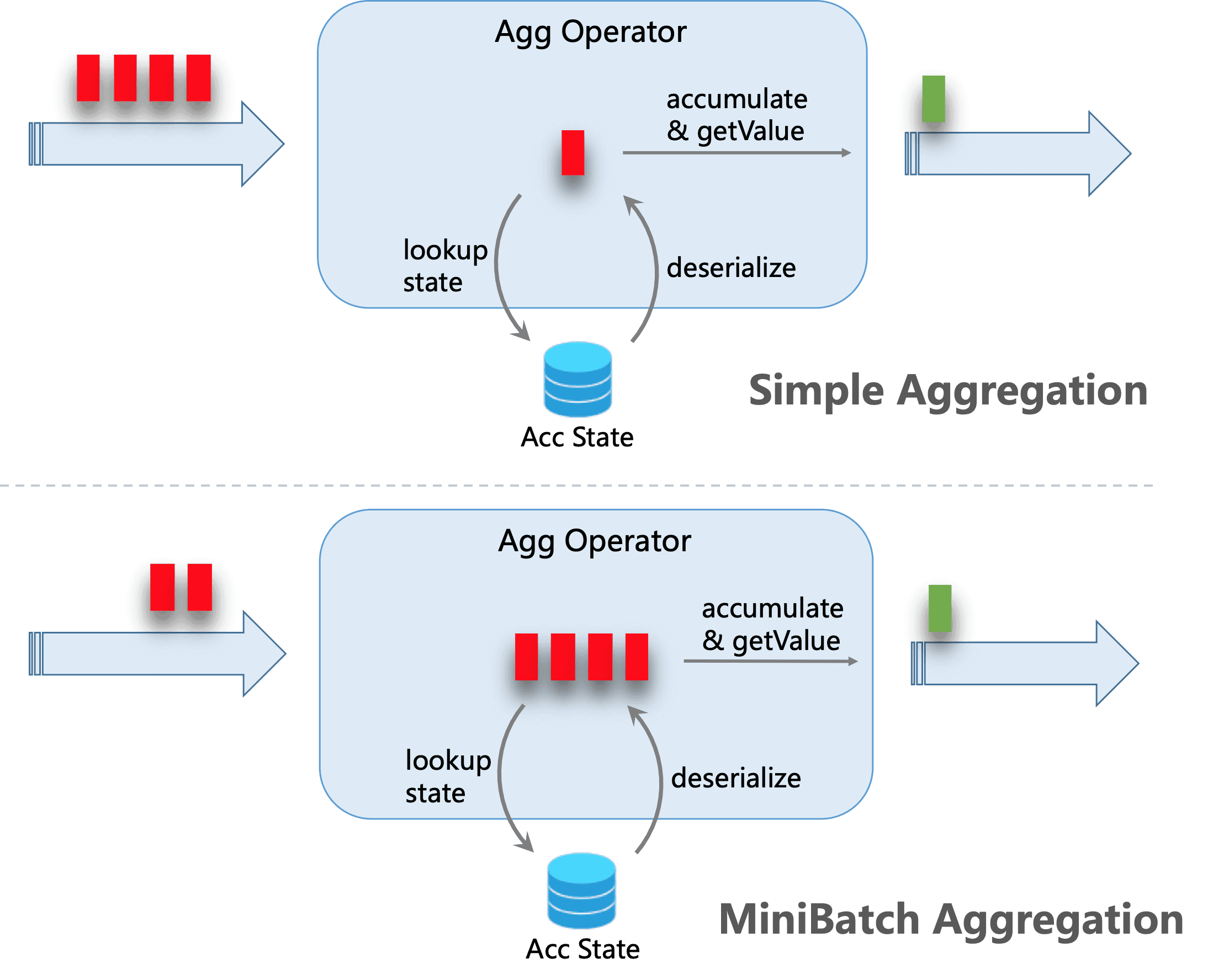
Mini batch optimization is disabled by default. To enable this optimization, you need to set the option table exec. mini-batch. enabled,table. exec. mini-batch. Allow latency and table exec. mini-batch. size.

// instantiate table environment
TableEnvironment tEnv = ...

// access flink configuration
Configuration configuration = tEnv.getConfig().getConfiguration();
// set low-level key-value options
configuration.setString("table.exec.mini-batch.enabled", "true"); // enable mini-batch optimization
configuration.setString("table.exec.mini-batch.allow-latency", "5 s"); // use 5 seconds to buffer input records
configuration.setString("table.exec.mini-batch.size", "5000"); // the maximum number of records can be buffered by each aggregate operator task

Local global aggregation

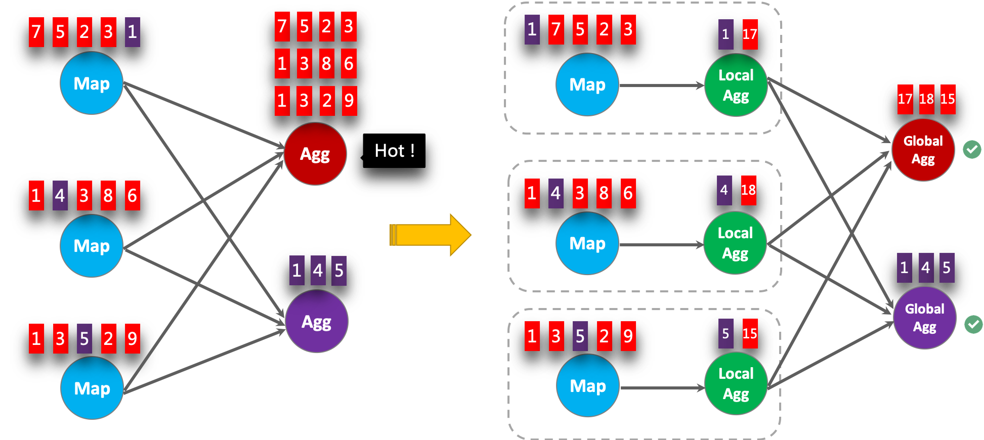
Local global aggregation is proposed to solve the problem of data skew. A group of aggregation is divided into two stages. First, local aggregation is carried out in the upstream, and then global aggregation is carried out in the downstream, which is similar to the Combine + Reduce mode in MapReduce. For example, for the following SQL:

SELECT color, sum(id) FROM T GROUP BY color

Records in the data stream may be skewed, so some instances of aggregation operators must process more records than others, which will cause hot issues. Local aggregation can accumulate a certain number of input data with the same key into a single accumulator. Global aggregation will only receive the reduced accumulator, not a large amount of original input data. This can greatly reduce the cost of network shuffle and state access. The amount of input data accumulated per local aggregation is based on the mini batch interval. This means that local global aggregation depends on enabling Mini batch optimization.

The following figure shows how local global aggregation can improve performance.

 

// instantiate table environment
TableEnvironment tEnv = ...

// access flink configuration
Configuration configuration = tEnv.getConfig().getConfiguration();
// set low-level key-value options
configuration.setString("table.exec.mini-batch.enabled", "true"); // local-global aggregation depends on mini-batch is enabled
configuration.setString("table.exec.mini-batch.allow-latency", "5 s");
configuration.setString("table.exec.mini-batch.size", "5000");
configuration.setString("table.optimizer.agg-phase-strategy", "TWO_PHASE"); // enable two-phase, i.e. local-global aggregation

Split distinct aggregation

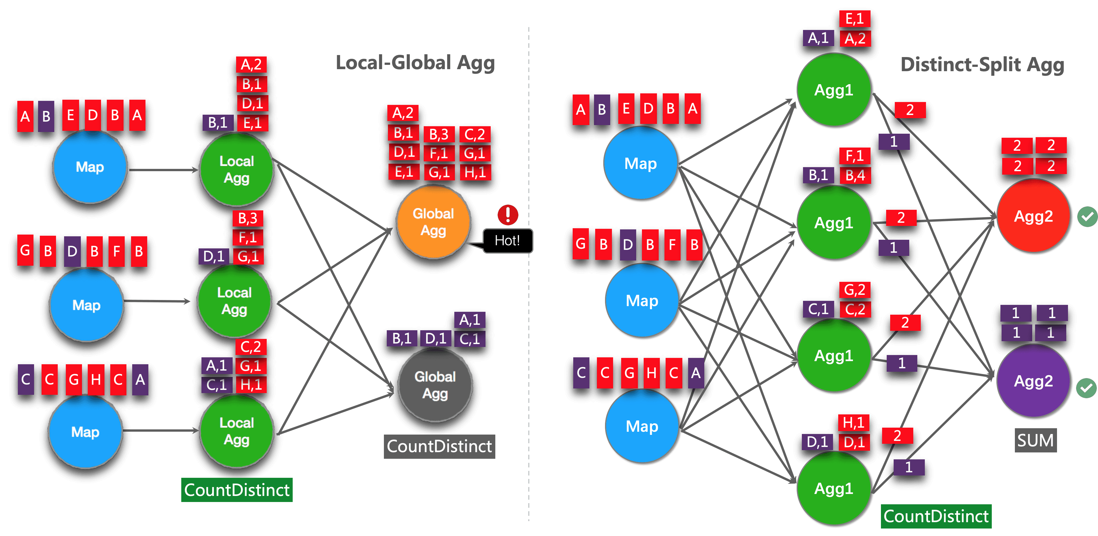
Local global optimization can effectively eliminate the data skew of conventional aggregation, such as SUM, COUNT, MAX, MIN and AVG. However, when dealing with distinct aggregation, its performance is not satisfactory.

For example, if we want to analyze how many unique users are logged in today. We may have the following queries:

SELECT day, COUNT(DISTINCT user_id) FROM T GROUP BY day

If the value distribution of distinct key (i.e. user_id) is sparse, COUNT DISTINCT is not suitable for reducing data. Even if local global optimization is enabled, it doesn't help much. Because the accumulator still contains almost all the original records, and global aggregation will become a bottleneck (most heavy accumulators are processed by one task, that is, the same day).

The idea of this optimization is to divide different aggregations (e.g. COUNT(DISTINCT col)) into two levels. The first aggregation is shuffle d by group key and additional bucket key. Bucket key uses {HASH_CODE(distinct_key) % BUCKET_NUM = calculated. BUCKET_NUM ， defaults to 1024, which can be accessed through ， table optimizer. distinct-agg. split. Bucket num option. The second aggregation is performed by shuffling the original group key and aggregating the COUNT DISTINCT values from different buckets using SUM. Since the same distinct key will only be calculated in the same bucket, the conversion is equivalent. Bucket key acts as an additional group key to share the burden of hotspots in group key. Bucket key makes job s scalable to solve data skew / hot spots in different aggregations.

After splitting distinct aggregation, the above query will be automatically rewritten into the following query:

SELECT day, SUM(cnt)
FROM (
    SELECT day, COUNT(DISTINCT user_id) as cnt
    FROM T
    GROUP BY day, MOD(HASH_CODE(user_id), 1024)
)
GROUP BY day

The following figure shows how splitting distinct aggregates improves performance (assuming that colors represent days and letters represent user_id).

Note: the above is the simplest example that can benefit from this optimization. In addition, Flink also supports splitting more complex aggregate queries. For example, multiple distinct aggregations with different distinct key s (e.g., COUNT(DISTINCT a), SUM(DISTINCT b)) can be used together with other non distinct aggregations (e.g., COUNT, MAX, MIN, COUNT).

Note: Currently, split optimization does not support aggregatefunctions that contain user-defined aggregatefunctions.

// instantiate table environment
TableEnvironment tEnv = ...

tEnv.getConfig()        // access high-level configuration
  .getConfiguration()   // set low-level key-value options
  .setString("table.optimizer.distinct-agg.split.enabled", "true");  // enable distinct agg split

Use the FILTER modifier on a distinct aggregate

In some cases, users may need to calculate the number of UVs (independent visitors) from different dimensions, such as UVs from Android, iPhone, Web and total UVs. Many people choose CASE WHEN, for example:

SELECT
 day,
 COUNT(DISTINCT user_id) AS total_uv,
 COUNT(DISTINCT CASE WHEN flag IN ('android', 'iphone') THEN user_id ELSE NULL END) AS app_uv,
 COUNT(DISTINCT CASE WHEN flag IN ('wap', 'other') THEN user_id ELSE NULL END) AS web_uv
FROM T
GROUP BY day

However, in this case, it is recommended to use the {FILTER} syntax instead of CASE WHEN. Because FILTER is more in line with SQL standards and can get more performance improvements. FILTER ， is a modifier for aggregation functions that limits the values used in aggregation. Replace the above example with the FILTER modifier as follows:

SELECT
 day,
 COUNT(DISTINCT user_id) AS total_uv,
 COUNT(DISTINCT user_id) FILTER (WHERE flag IN ('android', 'iphone')) AS app_uv,
 COUNT(DISTINCT user_id) FILTER (WHERE flag IN ('wap', 'other')) AS web_uv
FROM T
GROUP BY day

The Flink SQL optimizer can recognize different filter parameters on the same distinct key. For example, in the above example, all three COUNT DISTINCT are in user_id ， on a column. Flink can use only one shared state instance instead of three state instances to reduce state access and state size. Significant performance gains can be achieved under certain workloads.

Currently, the blogger specializes in real-time computing and computing platform research and development, and has the background of communication industry and e-commerce industry. He is familiar with Flink Spark computing engine and OLAP complex query. Welcome to add wechat and communicate together