1, Algorithm requirements

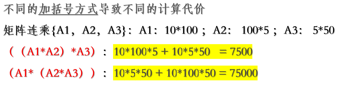
Given n matrices {A, A, A,,..., An}, where Ai and Ai + 1 (I = 1, 2,..., n-1) are multiplicative. The order of matrix multiplication is expressed by the method of adding brackets. The calculation amount (multiplication times) is different in different calculation orders. Find A method of adding brackets to minimize the calculation amount of matrix multiplication.

1. Ideas

Given n matrices {A1,A2,..., an}, where a and Ai+1 are multiplicative (i=1,2,..., n-1). Consider the continued product A1A2... An of these n matrices. Because the matrix multiplication satisfies the association law, the continued product of the matrix can be calculated in different orders.
This calculation order can be determined in parentheses. If the calculation order of a matrix continued product is completely determined, that is, the continued product has been completely bracketed, the standard algorithm for multiplying two matrices can be repeatedly called in this order to calculate the matrix continued product.
The fully bracketed matrix continued product can be recursively defined as:
① A single matrix is completely bracketed;
② If the matrix continued product A is completely bracketed, then A can be expressed as the product of two completely bracketed matrix continued products B and C and bracketed, that is, A=(BC).

	For example, matrix continued product A1A2A3A4 There are five complete bracketed methods:
	(A1(A2(A3A4))),(A1((A2A3)A4)),((A1A2)(A3A4)),((A1(A2A3))A4),(((A1A2)A3)A4)
	Each completely bracketed method corresponds to a calculation order of matrix continued product, and the calculation order of matrix continued product is closely related to its calculation amount.
	First, consider the amount of computation required to calculate the product of two matrices.
	The standard algorithm for calculating the product of two matrices is as follows, where, ra,ca and rb,cb Matrix representation A and B Number of rows and columns.

2. Examples

2, Complete code

1. Master file

main.cpp:

// Project1: matrix continued multiplication

#include<iostream>
using namespace std; 

const int rangeMatrix = 100;
int p[rangeMatrix];					//Row column array
int m[rangeMatrix][rangeMatrix],	//Result array
	s[rangeMatrix][rangeMatrix];	//Breakpoint array
int n;

// n = 5
// p[] = {3 5 10 8 2 4}

void Print(int i, int j) {
	if (i == j) {
		cout << "A["
			<< i << "]";
		return;
	}
	cout << "(";
	Print(i, s[i][j]);
	Print(s[i][j] + 1, j);
	cout << ")";
}

void MatrixChain() {
	int i, j, r, k;
	memset(m, 0, sizeof(m));	
	memset(s, 0, sizeof(s));	//Initialize array element to 0
	for (r = 2; r <= n; r++) {	//Subproblems of different sizes
		for (i = 1; i <= n - r + 1; i++) {
			j = i + r - 1;
			m[i][j] = m[i + 1][j] + p[i - 1] * p[i] * p[j];//Multiplication times with decision k=i
			s[i][j] = i;					//The optimal strategy of the subproblem is i
			for (k = i + 1; k < j; k++) {	//For all decisions from i to j, find the optimal value and record the optimal strategy{
				int t = m[i][k] + m[k + 1][j] + p[i - 1] * p[k] * p[j];
				if (t < m[i][j]) {
					m[i][j] = t;
					s[i][j] = k;
				}
			}
		}
	}
}

int main() {
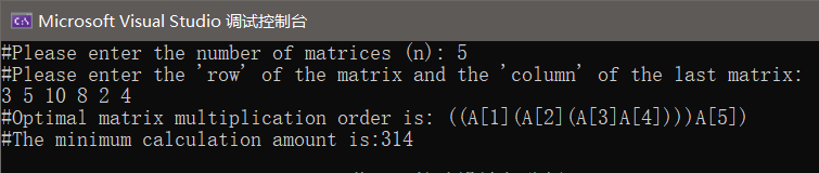
	cout << "#Please enter the number of matrices (n): ";
	cin >> n;
	cout << "#Please enter the 'row' of the matrix "
		<< "and the 'column' of the last matrix: ";
	int i, j;
	for (i = 0; i <= n; i++) {
		cin >> p[i];
	}
	MatrixChain();
	cout << "#Optimal matrix multiplication order is: ";
	Print(1, n);
	cout << "\n#The minimum calculation amount is:" 
		<< m[1][n] << endl;
	return 0;
}

2. Effect display

3, Supplement

Operation example of MatrixChain:

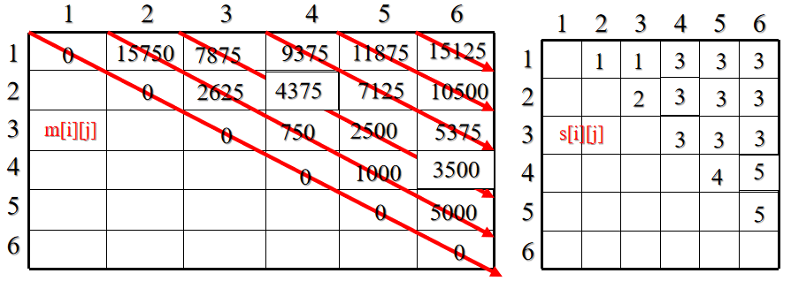
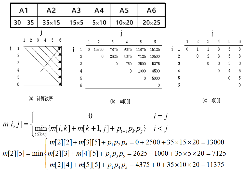
from m[1][6]=15125 It can be seen that the minimum number of operations of the continuous product of these six matrices is 15125.
from s[1][6] = 3 knowable A[1: 6]The optimal calculation order is A[1: 3] A[4: 6]；
from s[1][3] = 1 knowable A[1: 3]The optimal calculation order is A[1: 1] A[2: 3]；
from s[4][6] = 5 knowable A[4: 6]The optimal calculation order is A[4: 5] A[6: 6]；
Therefore, the optimal calculation order is:(A1(A2A3))((A4A5)A6). 

Algorithm complexity analysis:
(1) Time complexity:
It can be concluded from the program that the statement t=m[i][k] + m[k+1][j]+p[i-1]*p[k]*p[j], which is the basic statement of the algorithm and is nested in a three-tier for loop. In the worst case, the execution times of the statement is O(n3), the time of the print() function algorithm mainly depends on recursion, and the time complexity is O(n). Therefore, the time complexity of the program is O(n3).
(2) Space complexity:
The array of input data of the program is p [], and the auxiliary variables are i, j, r, t, k, m[]I], s [] []. The spatial complexity depends on the auxiliary space, so the spatial complexity is O(n2).

The document is for my study notes and is only for reference.