Authors: Chen Yingxiang, Yang Zihan
Compilation: AI Youdao
After data preprocessing, we generate a large number of new variables (for example, single hot coding generates a large number of variables containing only 0 or 1). But in fact, some newly generated variables may be redundant: on the one hand, they do not necessarily contain useful information, so they can not improve the performance of the model; On the other hand, these redundant variables will consume a lot of memory and computing power when building the model. Therefore, we should select features and select feature subsets for modeling.
Project address:
https://github.com/YC-Coder-Chen/feature-engineering-handbook/blob/master/%E4%B8%AD%E6%96%87%E7%89%88.md
This paper will introduce the Wrapper Methods encapsulation method in feature engineering.
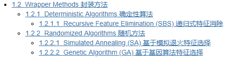
catalog:
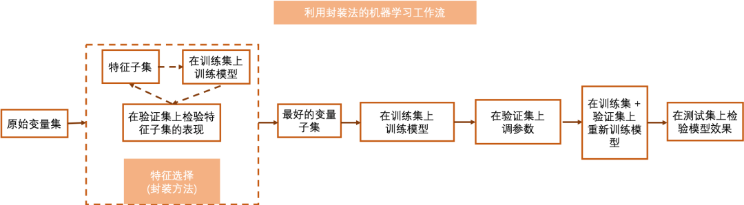
The encapsulation method regards the feature selection problem as a search problem, that is, its goal is to search for an optimal subset from the feature subset set, and this subset performs best in the model. In each step, it trains the model on the feature subset and then evaluates it. In the next step, it continues to adjust the feature subset and retrain the evaluation until the best subset is found or the maximum number of iterations is reached. Exhaustive search is NP hard in the packaging method, so some methods are proposed to reduce the number of iterations required by the packaging method, so that a better effect can be achieved in a limited time.
1.2.1 Deterministic Algorithms
Without considering the randomness of the model, given the same data input, the deterministic algorithm will always output the same optimal feature subset.
Sequential forward selection (SFS) and sequential backward selection (SBS) are deterministic algorithms. Sequential forward selection (SFS) method will start from the optimal univariate model, and then in the iteration, it will add a new variable to the existing variable subset by exhaustive method based on the variable quantum set in the previous step, so that the variable subset after adding a new variable can obtain the maximum improvement of model performance. The iteration will continue until the number of selected variables meets the requirements.
Sequential backward selection (SBS) starts from a model containing all variables, and then in the iteration, it will delete a variable with the lowest negative impact on the model in the existing variable subset by exhaustive method based on the variable quantum set in the previous step until the number of selected features meets the requirements.
However, both sequential forward selection (SFS) and sequential backward selection (SBS) are step wise methods, which may fall into local optimal state.
1.2.1.1 Recursive Feature Elimination (SBS)
In sklearn, it only implements the recursive feature elimination (SBS) method. It provides two functions to implement this method, one is RFE and the other is RFECV. Compared with RFE function, REFCV uses the results of cross validation to select the optimal number of features, while in RFE, the number of features to be selected is predefined by the user.
# RFE function demonstration
import numpy as np
from sklearn.feature_selection import RFE


# Load dataset directly
from sklearn.datasets import fetch_california_housing
dataset = fetch_california_housing()
X, y = dataset.data, dataset.target # Using california_housing dataset to demonstrate


# Select the first 15000 observation points as the training set
# The rest are used as test sets
train_set = X[0:15000,:]
test_set = X[15000:,]
train_y = y[0:15000]


# Select a supervised machine learning model to measure subset performance
from sklearn.ensemble import ExtraTreesRegressor # Use the ExtraTrees model as an example
clf = ExtraTreesRegressor(n_estimators=25)
selector = RFE(estimator = clf, n_features_to_select = 4, step = 1)
# Different from RFECV, the RFE function here requires the user to define the number of variables to be selected. It is set here to select four best variables, and we only delete one variable in each step


selector = selector.fit(train_set, train_y) # Train on the training set


transformed_train = train_set[:,selector.support_]  # Transform training set
assert np.array_equal(transformed_train, train_set[:,[0,5,6,7]]) # The first, sixth, seventh and eighth variables were selected


transformed_test = test_set[:,selector.support_] # Transform training set
assert np.array_equal(transformed_test, test_set[:,[0,5,6,7]]) # The first, sixth, seventh and eighth variables were selected
# RFECV function demonstration
import numpy as np
from sklearn.feature_selection import RFECV


# Load dataset directly
from sklearn.datasets import fetch_california_housing
dataset = fetch_california_housing()
X, y = dataset.data, dataset.target # Using california_housing dataset to demonstrate


# Select the first 15000 observation points as the training set
# The rest are used as test sets
train_set = X[0:15000,:]
test_set = X[15000:,]
train_y = y[0:15000]


# Select a supervised machine learning model to measure subset performance
from sklearn.ensemble import ExtraTreesRegressor # Use the ExtraTrees model as an example
clf = ExtraTreesRegressor(n_estimators=25)
selector = RFECV(estimator = clf, step = 1, cv = 5) # Use 50% off cross validation
# At each step, we delete only one variable
selector = selector.fit(train_set, train_y)


transformed_train = train_set[:,selector.support_]  # Transform training set
assert np.array_equal(transformed_train, train_set) # All variables are selected


transformed_test = test_set[:,selector.support_] # Transform training set
assert np.array_equal(transformed_test, test_set) # All variables are selected
1.2.2 Randomized Algorithms
Compared with deterministic algorithm, stochastic method introduces a certain degree of randomness in searching the best feature subset. Therefore, in the case of the same data input, it may output different optimal feature subset results, but the randomness in this method will help to avoid the model falling into local optimal results.
1.2.2.1 Simulated Annealing (SA) feature selection based on simulated annealing
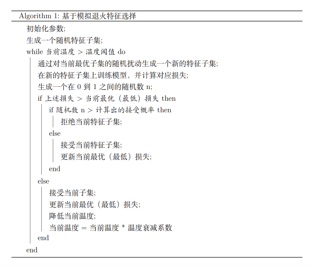
Simulated annealing is a stochastic optimization method, which has been introduced into the field of feature selection in recent years. In each step, we will randomly select a feature subset according to the current optimal feature subset. If the new feature subset works better, we will adopt it and update the current optimal feature subset. If the new feature subset performs poorly, we will still accept it with a certain probability, which depends on the current state (temperature).
It is very important for simulated annealing algorithm to accept the feature subset with poor realization with a certain probability, because it helps the algorithm to avoid falling into local optimal state. With the iteration, the simulated annealing algorithm can converge to a good and stable final result.
Since no function that can better implement SA algorithm is found, I have written a python script to implement SA algorithm for your reference. It can be well compatible with the models in sklearn and support classification and regression problems. It also provides built-in cross validation methods.
Formula:
In each step, the probability of accepting the feature subset with poor performance is:
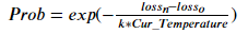
Prob is the probability of accepting a subset of features with poor performance???????????????????? Is the loss of the new feature subset???????????????????? For the optimal (minimum) loss before creating a new feature subset, you can???????????????????????????????????????????? Is the current temperature. Pseudo code of simulated annealing is:
Regression problem demonstration
import sys
sys.path.append("..")
from SA import Simulated_Annealing # Import the module we wrote


# Load dataset directly
from sklearn.datasets import fetch_california_housing
dataset = fetch_california_housing()
X, y = dataset.data, dataset.target # Using california_housing dataset to demonstrate


# Select the first 15000 observation points as the training set
# The rest are used as test sets
train_set = X[0:15000,:]
test_set = X[15000:,]
train_y = y[0:15000]


# Select a supervised machine learning model to measure subset performance
from sklearn.ensemble import ExtraTreesRegressor # Use the ExtraTrees model as an example


# Select the loss function of evaluation feature subset in simulated annealing
from sklearn.metrics import mean_squared_error # For regression problems, we use MSE


clf = ExtraTreesRegressor(n_estimators=25)
selector = Simulated_Annealing(loss_func = mean_squared_error, estimator = clf,
                               init_temp = 0.2, min_temp = 0.005, iteration = 10, alpha = 0.9)
# Focus on training
# SA.py has the meaning of each parameter, which will not be repeated here


selector.fit(X_train = train_set, y_train = train_y, cv = 5) # Use 50% off cross validation


transformed_train = selector.transform(train_set) # Transform training set
transformed_test = selector.transform(test_set)  # Transform test set
selector.best_sol # Returns the index of the best feature selector.best_loss; # Returns the loss corresponding to the optimal feature subset
Classification problem presentation
import sys
sys.path.append("..")
import numpy as np
import random
from SA import Simulated_Annealing # Import the module we wrote


from sklearn.datasets import load_iris  # Using iris data as demonstration data set


# Load dataset
iris = load_iris()
X, y = iris.data, iris.target


# iris datasets need to be out of order before use
np.random.seed(1234)
idx = np.random.permutation(len(X))
X = X[idx]
y = y[idx]


# Select the first 100 observation points as the training set
# The remaining 20 observation points are used as the verification set and the remaining 30 observations are used as the test set
train_set = X[0:100,:]
val_set = X[100:120,:]
test_set = X[120:,:]


train_y = y[0:100]
val_y = y[100:120]
test_y = y[120:]


# Reproducing random seeds
# Stochastic methods require the existence of randomness
random.seed()
np.random.seed()


# Select a supervised machine learning model to measure subset performance
from sklearn.ensemble import ExtraTreesClassifier # we use extratree as predictive model


# Select the loss function of evaluation feature subset in simulated annealing
from sklearn.metrics import log_loss # In the regression problem, we use the cross entropy loss function


clf = ExtraTreesClassifier(n_estimators=25)
selector = Simulated_Annealing(loss_func = log_loss, estimator = clf,
                               init_temp = 0.2, min_temp = 0.005, iteration = 10,
                               alpha = 0.9, predict_type = 'predict_proba')
# Focus on training
# SA.py has the meaning of each parameter, which will not be repeated here


selector.fit(X_train = train_set, y_train = train_y, X_val = val_set,
             y_val = val_y, stop_point = 15)
# This function allows users to import their own defined validation sets. Try it here


transformed_train = selector.transform(train_set)  # Transform training set
transformed_test = selector.transform(test_set)  # Transform test set
selector.best_sol # Returns the index of the best feature selector.best_loss; # Returns the loss corresponding to the optimal feature subset
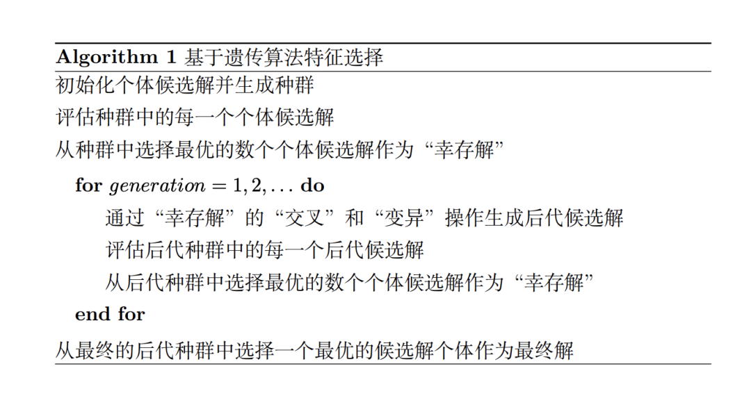
1.2.2.2 Genetic Algorithm (GA) feature selection based on genetic algorithm
Genetic algorithm is an optimization search algorithm based on the concept of evolutionary biology. It draws lessons from the evolution process in nature, and allows individual candidate solutions to evolve through "crossover" and "mutation" to obtain better candidate solutions and populations. It also combines the concept of competition in nature, that is, only the most appropriate or optimal candidate solutions are allowed to "survive" and "reproduce" their offspring. After continuous iteration of population and individual candidate solutions, genetic algorithm (GA) will converge to the optimal solution.
Similar to simulated annealing, I also wrote a python script to implement GA algorithm for your reference. It provides two algorithms, including "one Max" and "NSGA2". "One Max" is a traditional single objective GA algorithm, and "NSGA2" is a multi-objective GA algorithm. In feature selection, the goal of "one Max" is to reduce the loss of simulation on the verification set, while the goal of "NSGA2" is to reduce the loss and minimize the number of features in the feature subset at the same time.
This python script is well compatible with the model in sklearn and supports classification and regression problems. It also provides built-in cross validation methods.
The pseudocode of genetic algorithm is as follows:
Regression problem demonstration
import sys
sys.path.append("..")
from GA import Genetic_Algorithm # Import the module we wrote


# Load dataset directly
from sklearn.datasets import fetch_california_housing
dataset = fetch_california_housing()
X, y = dataset.data, dataset.target # Using california_housing dataset to demonstrate


# Select the first 15000 observation points as the training set
# The rest are used as test sets
train_set = X[0:15000,:]
test_set = X[15000:,]
train_y = y[0:15000]


# Select a supervised machine learning model to measure subset performance
from sklearn.ensemble import ExtraTreesRegressor # Use the ExtraTrees model as an example


# Select the loss function of evaluation feature subset in simulated annealing
from sklearn.metrics import mean_squared_error # For regression problems, we use MSE


clf = ExtraTreesRegressor(n_estimators=25)
selector = Genetic_Algorithm(loss_func = mean_squared_error, estimator = clf,
                             n_gen = 10, n_pop = 20, algorithm = 'NSGA2')
# Focus on training
# GA.py has the specific meaning of each parameter, which will not be repeated here


selector.fit(X_train = train_set, y_train = train_y, cv = 5) # Use 50% off cross validation


transformed_train = selector.transform(train_set) # Transform training set
transformed_test = selector.transform(test_set)  # Transform test set
selector.best_sol # Returns the index of the best feature selector.best_loss; # Returns the loss corresponding to the optimal feature subset
Classification problem presentation
import sys
sys.path.append("..")
import numpy as np
import random
from GA import Genetic_Algorithm # Import the module we wrote


from sklearn.datasets import load_iris  # Using iris data as demonstration data set


# Load dataset
iris = load_iris()
X, y = iris.data, iris.target


# iris datasets need to be out of order before use
np.random.seed(1234)
idx = np.random.permutation(len(X))
X = X[idx]
y = y[idx]


# Select the first 100 observation points as the training set
# The remaining 20 observation points are used as the verification set and the remaining 30 observations are used as the test set
train_set = X[0:100,:]
val_set = X[100:120,:]
test_set = X[120:,:]


train_y = y[0:100]
val_y = y[100:120]
test_y = y[120:]


# Reproducing random seeds
# Stochastic methods require the existence of randomness
random.seed()
np.random.seed()


# Select a supervised machine learning model to measure subset performance
from sklearn.ensemble import ExtraTreesClassifier # we use extratree as predictive model


# Select the loss function of evaluation feature subset in simulated annealing
from sklearn.metrics import log_loss # In the regression problem, we use the cross entropy loss function


clf = ExtraTreesClassifier(n_estimators=25)
selector = Genetic_Algorithm(loss_func = log_loss, estimator = clf,
                             n_gen = 15, n_pop = 10, predict_type = 'predict_proba')
# Focus on training
# GA.py has the specific meaning of each parameter, which will not be repeated here


selector.fit(X_train = train_set, y_train = train_y, X_val = val_set,
             y_val = val_y, stop_point = 15)
# This function allows users to import their own defined validation sets. Try it here


transformed_train = selector.transform(train_set)  # Transform training set
transformed_test = selector.transform(test_set)  # Transform test set
selector.best_sol # Returns the index of the best feature selector.best_loss; # Returns the loss corresponding to the optimal feature subset
Chinese Jupyter address:
https://github.com/YC-Coder-Chen/feature-engineering-handbook/tree/master/%E4%B8%AD%E6%96%87%E7%89%88