Whether using all variables or the selected characteristic variables, and no matter how the cross validation parameters are adjusted, the prediction accuracy of the model obtained when applied to the test set can be more than 90%, but compared with the random guess based on no information, This model is not statistically significant (this may not be significant, and the overall accuracy of the model is meaningless when the sample is unbalanced). One reason should be the sample imbalance. The number of samples in DLBCL group was about 3 times that in FL group. 75% accuracy can be obtained without modeling but only blind guessing that the result is DLBCL. The prediction accuracy of FL group is very low.
Usually, we focus on a small number of samples, such as whether they are ill. We prefer to find possible diseases and take measures in advance.
Therefore, how to deal with non-equilibrium samples needs to be considered when each algorithm is applied to classification problems.
The impact of unbalanced samples in the model construction is mainly reflected in two places:
- When building a decision tree by random sampling, there will be a high probability that only the classification with more samples will be obtained. These trees will not be able to predict the classification with less samples, so as to form a meaningless decision tree.
- The decisions made at each molecular node of the decision tree tend to the overall classification purity, so the classification with less samples has less contribution and impact on the results.
There are four general processing methods:
- Class weights: impose a higher cost when errors are made in the minor class
- Down sampling: randomly remove samples from classes with many samples
- Up sampling: randomly replicate instances in the minority class
- Synthetic minor sampling technique (smote): synthesize filled samples in classes with few samples by interpolation
These weight weighting or sampling techniques have a great impact on the threshold dependent evaluation indicators such as accuracy. They are equivalent to pushing the decision threshold to the "optimal position" in the ROC curve (which is described in the Boruta characteristic variable screening part). However, these weight weighting or sampling techniques usually have little impact on the ROC curve.
Sample imbalance processing based on simulated data
Here, first get familiar with the processing flow through a set of simulated data, and then apply it to real data. The twoClassSim function of caret package is used to generate a data set containing 20 meaningful variables and 10 noise variables. The data set contains 5000 observation samples and is divided into two groups. The proportion of the number of samples in most groups and a few groups is 50:1 (controlled by intercept parameter).
library(dplyr) # for data manipulation
library(caret) # for model-building
# install.packages("xts")
# install.packages("quantmod")
# wget https://cran.r-project.org/src/contrib/Archive/DMwR/DMwR_0.4.1.tar.gz
# R CMD INSTALL DMwR_0.4.1.tar.gz
library(DMwR) # for smote implementation
# Or use smotefamily instead
# library(smotefamily) # for smote implementation
library(purrr) # for functional programming (map)
library(pROC) # for AUC calculations

set.seed(2969)

imbal_train <- twoClassSim(5000,
                           intercept = -25,
                           linearVars = 20,
                           noiseVars = 10)

imbal_train$Class = ifelse(imbal_train$Class == "Class1", "Normal", "Disease")
imbal_train$Class <- factor(imbal_train$Class, levels=c("Disease", "Normal"))

imbal_test  <- twoClassSim(5000,
                           intercept = -25,
                           linearVars = 20,
                           noiseVars = 10)
imbal_test$Class = ifelse(imbal_test$Class == "Class1", "Normal", "Disease")
imbal_test$Class <- factor(imbal_test$Class, levels=c("Disease", "Normal"))

prop.table(table(imbal_train$Class))

prop.table(table(imbal_test$Class))
Sample composition
Disease  Normal
 0.0204  0.9796

Disease  Normal
 0.0252  0.9748
Build original GBM model
Here, another integrated learning algorithm (GBM, Gradient Boosting Machine) is applied to build the model. GBM is also an effective ensemble learning algorithm, which can deal with the interaction and nonlinear relationship of variables. GBDT, XGBoost and LightGBM algorithms (or tools) commonly used in machine learning are based on the algorithm idea of gradient hoist (GBM).
Firstly, an original model is constructed, and the 10 fold cross validation is repeated five times to find the optimal model super parameters, and AUC is used as the evaluation standard. If you are not familiar with these concepts, turn to previous tweets.
# Set up control function for training
ctrl <- trainControl(method = "repeatedcv",
                     number = 10,
                     repeats = 5,
                     summaryFunction = twoClassSummary,
                     classProbs = TRUE)

# Build a standard classifier using a gradient boosted machine

set.seed(5627)
orig_fit <- train(Class ~ .,
                  data = imbal_train,
                  method = "gbm",
                  verbose = FALSE,
                  metric = "ROC",
                  trControl = ctrl)

# Build custom AUC function to extract AUC
# from the caret model object

test_roc <- function(model, data) {
  roc(data$Class,
      predict(model, data, type = "prob")[, "Disease"])

}

orig_fit %>%
  test_roc(data = imbal_test) %>%
  auc()
The AUC value is 0.95, which is still very good.
Setting levels: control = Disease, case = Normal
Setting direction: controls > cases
Area under the curve: 0.9538
According to the conflict matrix (default threshold is adopted for prediction results), the classification effect of Disease is general, and the accuracy (sensitivity) is only 30.6%. Both Normal and Disease tend to be predicted as Normal with low specificity, which is caused by sample imbalance. And we usually prefer to find the existence of the Disease as soon as possible.
predictions_train <- predict(orig_fit, newdata=imbal_test)
confusionMatrix(predictions_train, imbal_test$Class)
Confusion Matrix and Statistics

          Reference
Prediction Disease Normal
   Disease      38     17
   Normal       88   4857

               Accuracy : 0.979
                 95% CI : (0.9746, 0.9828)
    No Information Rate : 0.9748
    P-Value [Acc > NIR] : 0.02954

                  Kappa : 0.4109

 Mcnemar's Test P-Value : 8.415e-12

            Sensitivity : 0.3016
            Specificity : 0.9965
         Pos Pred Value : 0.6909
         Neg Pred Value : 0.9822
             Prevalence : 0.0252
         Detection Rate : 0.0076
   Detection Prevalence : 0.0110
      Balanced Accuracy : 0.6490

       'Positive' Class : Disease
Deal with sample imbalance by weight distribution or sampling
The GBM model applied here has a parameter weights, which can be used to set the weight of the sample; caret provides the sampling parameter in the trainControl function, which can be used for up sample and down sample, or any other algorithm sampling method (here, the smotefamily::SMOTE function is used for sampling).
# Create model weights (they sum to one)
# Give each observer a weight
class1_weight = (1/table(imbal_train$Class)[['Normal']]) * 0.5
class2_weight = (1/table(imbal_train$Class)[["Disease"]]) * 0.5
model_weights <- ifelse(imbal_train$Class == "Normal",
                        class1_weight, class2_weight)

# Use the same seed to ensure same cross-validation splits
ctrl$seeds <- orig_fit$control$seeds

# Build weighted model

weighted_fit <- train(Class ~ .,
                      data = imbal_train,
                      method = "gbm",
                      verbose = FALSE,
                      weights = model_weights,
                      metric = "ROC",
                      trControl = ctrl)

# Build down-sampled model

ctrl$sampling <- "down"

down_fit <- train(Class ~ .,
                  data = imbal_train,
                  method = "gbm",
                  verbose = FALSE,
                  metric = "ROC",
                  trControl = ctrl)

# Build up-sampled model

ctrl$sampling <- "up"

up_fit <- train(Class ~ .,
                data = imbal_train,
                method = "gbm",
                verbose = FALSE,
                metric = "ROC",
                trControl = ctrl)

# Build smote model
ctrl$sampling <- "smote"

smote_fit <- train(Class ~ .,
                   data = imbal_train,
                   method = "gbm",
                   verbose = FALSE,
                   metric = "ROC",
                   trControl = ctrl)
Calculate the AUC value of each model
# Examine results for test set

model_list <- list(original = orig_fit,
                   weighted = weighted_fit,
                   down = down_fit,
                   up = up_fit,
                   SMOTE = smote_fit)

model_list_roc <- model_list %>%
  map(test_roc, data = imbal_test)

model_list_roc %>%
  map(auc)
The AUC obtained by the sample weighted model is the highest, followed by up sample, smote and down sample. The results are higher than the original.
Setting levels: control = Disease, case = Normal
Setting direction: controls > cases
Setting levels: control = Disease, case = Normal
Setting direction: controls > cases
Setting levels: control = Disease, case = Normal
Setting direction: controls > cases
Setting levels: control = Disease, case = Normal
Setting direction: controls > cases
Setting levels: control = Disease, case = Normal
Setting direction: controls > cases
$original
Area under the curve: 0.9538

$weighted
Area under the curve: 0.9793

$down
Area under the curve: 0.9667

$up
Area under the curve: 0.9778

$SMOTE
Area under the curve: 0.9744
Draw the lower ROC curve to see the specific effect display of the lower model. The sample weighted model is better than all other models, and the effect of the original model is worse than other models when the false positive rate is 0-25%. A good model has a higher true positive rate at a lower false positive rate.
results_list_roc <- list(NA)
num_mod <- 1

for(the_roc in model_list_roc){

  results_list_roc[[num_mod]] <-
    data_frame(TPR = the_roc$sensitivities,
               FPR = 1 - the_roc$specificities,
               model = names(model_list)[num_mod])

  num_mod <- num_mod + 1

}

results_df_roc <- bind_rows(results_list_roc)

results_df_roc$model <- factor(results_df_roc$model,
                               levels=c("original", "down","SMOTE","up","weighted"))

# Plot ROC curve for all 5 models

custom_col <- c("#000000", "#009E73", "#0072B2", "#D55E00", "#CC79A7")

ggplot(aes(x = FPR,  y = TPR, group = model), data = results_df_roc) +
  geom_line(aes(color = model), size = 1) +
  scale_color_manual(values = custom_col) +
  geom_abline(intercept = 0, slope = 1, color = "gray", size = 1) +
  theme_bw(base_size = 18) + coord_fixed(1)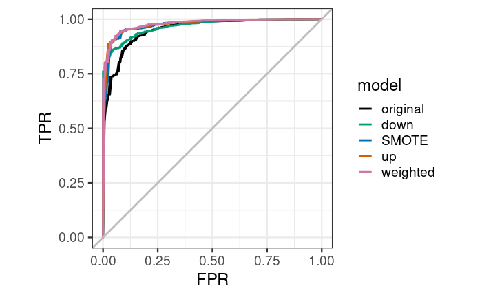
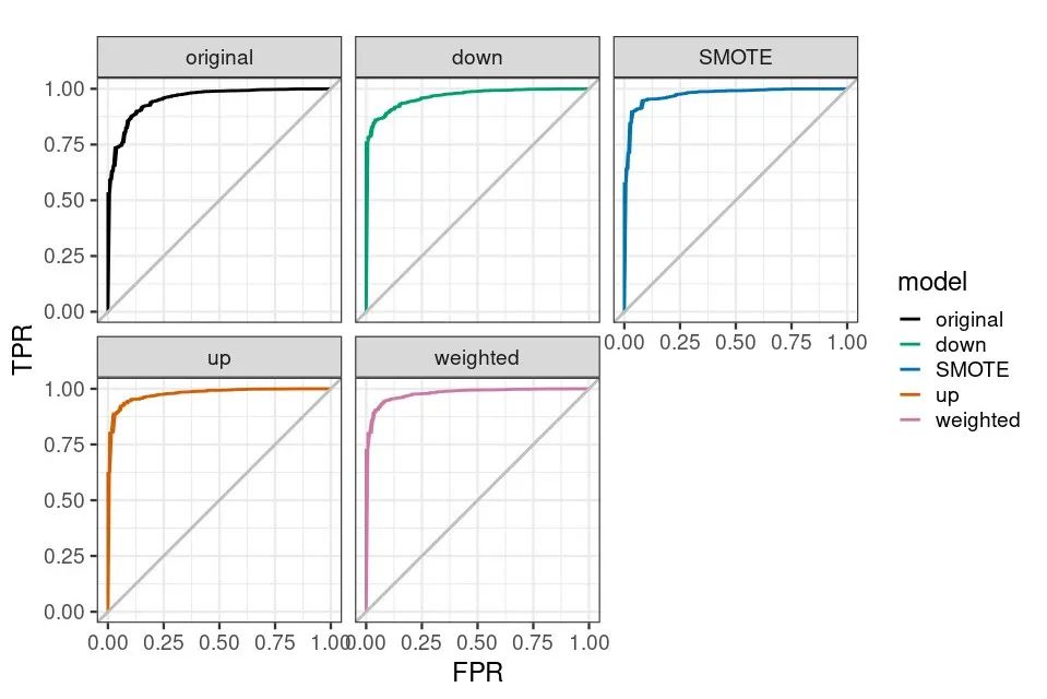
ggplot(aes(x = FPR,  y = TPR, group = model), data = results_df_roc) +
  geom_line(aes(color = model), size = 1) +
  facet_wrap(vars(model)) +
  scale_color_manual(values = custom_col) +
  geom_abline(intercept = 0, slope = 1, color = "gray", size = 1) +
  theme_bw(base_size = 18) + coord_fixed(1)
The total prediction accuracy of the weighted model decreased a little, but the prediction accuracy of Disease increased by 2.47 times, 70.63%.
predictions_train <- predict(weighted_fit, newdata=imbal_test)
confusionMatrix(predictions_train, imbal_test$Class)
give the result as follows
Confusion Matrix and Statistics

          Reference
Prediction Disease Normal
   Disease      89     83
   Normal       37   4791

               Accuracy : 0.976
                 95% CI : (0.9714, 0.9801)
    No Information Rate : 0.9748
    P-Value [Acc > NIR] : 0.3137

                  Kappa : 0.5853

 Mcnemar's Test P-Value : 3.992e-05

            Sensitivity : 0.7063
            Specificity : 0.9830
         Pos Pred Value : 0.5174
         Neg Pred Value : 0.9923
             Prevalence : 0.0252
         Detection Rate : 0.0178
   Detection Prevalence : 0.0344
      Balanced Accuracy : 0.8447

       'Positive' Class : Disease
From this set of test data, the model effect obtained by setting the weight is the best. But this is not absolute. When applying to your own data, you need to try to see which method your data is more suitable for.