Original link: http://tecdat.cn/?p=25067 

This paper describes how to} perform principal component analysis (PCA) using R. You will learn how to} use PCA_ Forecast_ New individual and variable coordinates. We will also provide_ PCA results_ The theory behind it.

There are two general methods to perform PCA in R:

• _ Spectral decomposition_ , check the covariance / correlation between variables
• The covariance / correlation between individuals was examined_ Singular value decomposition_

With the help of R, the numerical accuracy of SVD is slightly better.

visualization

Create an elegant visualization based on ggplot2.

Presentation dataset

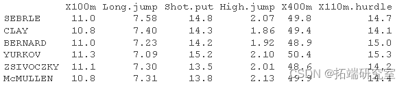
We will use the performance data set of athletes in Decathlon. The data used here describe the performance of athletes in two sports events

Data Description:
A data frame containing 27 observations of the following 13 variables.

X100m
A number vector

long jump
A number vector

shoot
A number vector

High jump
A number vector

X400m
Digital vector

X110m.hurdle
A number vector

Flying saucer
A number vector

Pole vault
A number vector

rope
Digital vector

X1500 m
Digital vector

level
Numeric vector corresponding to level

spot
A numeric vector that specifies the number of points obtained

sports meeting
Horizontal variable decimal olympicg

In short, it includes:

• Training individuals (rows 1 to 23) and training variables (columns 1 to 10) were used to perform principal component analysis
• The coordinates of the predicted individual (lines 24 to 27) and the predicted variable (columns 11 to 13) will be predicted using PCA information and parameters obtained by training the individual / variable.

Load data and extract only trained individuals and variables:

                       head(dec)

Calculate PCA

In this section, we will visualize PCA.

1. Visualization
2. Calculate PCA

prcomp

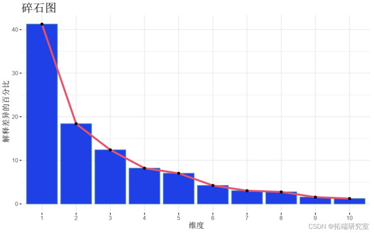
1. Visualization_ Eigenvalue_ (gravel diagram). Displays the percentage of variance explained by each principal component.

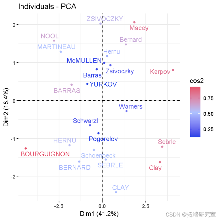
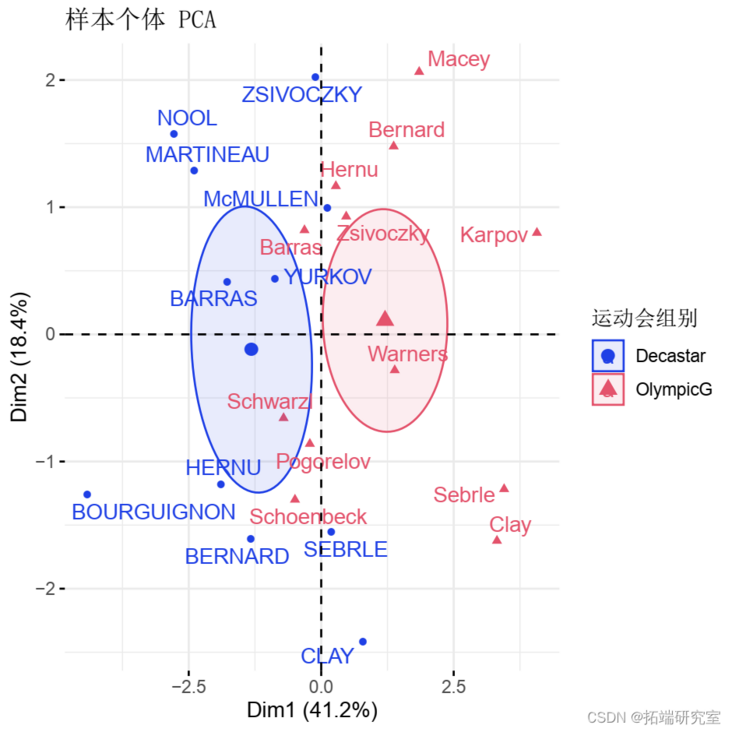
1. Individuals with similar characteristics were grouped.

viz(res )

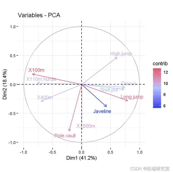
1. Variable diagram. Positive correlation variables point to the same side of the graph. Negative correlation variables point to the opposite sides of the chart.

vzpca(res )

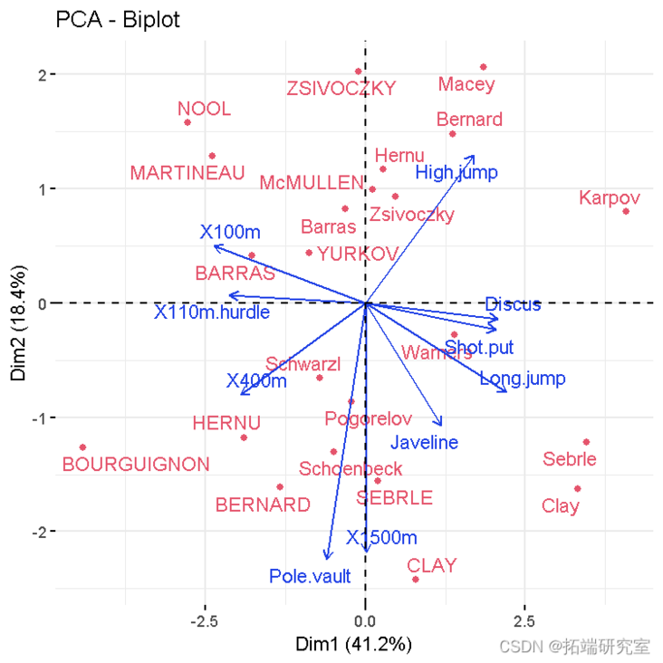
1. Double plot of individuals and variables

fvbiplot(res )

PCA results

#Eigenvalue
eigva

  
#Results of variables
coord #Coordinates
contrib #Contribution to PC
cos2 #Representative quality
#Personal results
coord #Coordinates
contrib #Contribution to PC
cos2 #Representative quality

Prediction using PCA

In this section, we will show how to use only the information provided by the previously performed PCA to predict the coordinates of supplementary individuals and variables.

Forecast individual

1. Data: rows 24 to 27 and columns 1 to 10. The new data must contain columns (variables) with the same name and order as the activity data used to calculate PCA.

#Predicting individual data
in <- dec\[24:27, 1:10\]

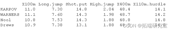
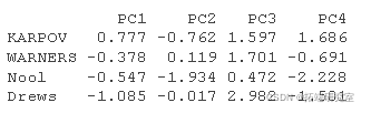
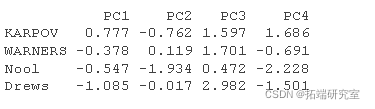
1. Predict the coordinates of the new individual data. Use R basis function_ predict_ ():

predict

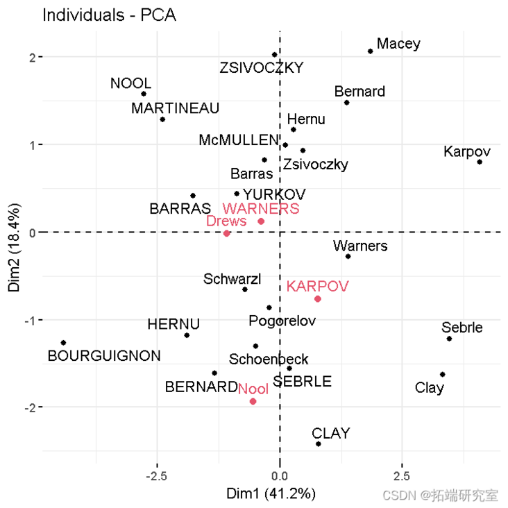
1. Personal chart including supplementary individuals:

#Atlas of active individuals
fvca_
#Add supplementary individual
fdd(p)

The individual prediction coordinates can be calculated as follows:

1. Centralize and standardize new personal data using the center and proportion of PCA
2. The prediction coordinates are calculated by multiplying the normalized value by the eigenvector (load) of the principal component.

You can use the following R Code:

#The supplementary individuals were centered and standardized
ined <- scale
#Individual coordinates

rtaton
ird <- t(apply)

Supplementary variable

Qualitative / categorical variables

The data set} contains the data corresponding to the type of competition in column 13_ Supplementary qualitative variables_  .

Qualitative / categorical variables can be used to color samples by group. The length of grouped variables should be the same as the number of active individuals.

groups <- as.factor
fvnd(res.pca
             )

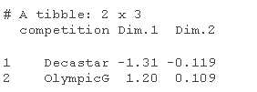
Calculate the horizontal coordinates of the grouped variables. The coordinates of a given group are calculated as the average coordinates of the individuals in the group.

library(magrittr) #Pipeline function% >%.
# 1. Single coordinate
getind(res)
# 2. Coordinates of the group
coord %>% >
  as\_data\_frame%>%
  selec%>%
  mutate%>%
  group_b %>%

Quantitative variable

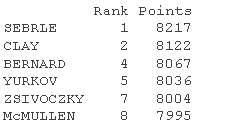
Data: column 11:12. It should be the same as the number of active individuals (23 here)

quup <- dec\[1:23, 11:12\]
head(quup .sup)

The coordinates of a given quantitative variable are calculated as the correlation between the quantitative variable and the principal component.

#Predict coordinates and calculate cos2
quaord <- cor
quaos2 <- qord^2
#Graphics of variables, including supplementary variables
p <- fviar(reca)
fvdd(p, quord, color ="blue", geom="arrow")

Theory behind PCA results

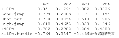
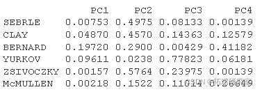
PCA results of variables

Here, we will show how to calculate the PCA results of variables: coordinates, cos2 and contribution:

• var.coord = standard deviation of load * component
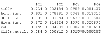
• var.cos2 = var.coord ^ 2
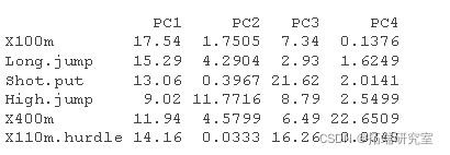
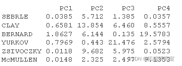
• var.contrib. The contribution of the variable to a given principal component is (percentage): (var.cos2 * 100) / (total Cos2 of the component)

#Calculate coordinates
#::::::::::::::::::::::::::::::::::::::::
logs <- rotation
sdev <- sdev
vad <- t(apply)

#Calculate Cos2
#::::::::::::::::::::::::::::::::::::::::
vaos2 <- vard^2
head(vars2\[, 1:4\])

#Calculated contribution
#::::::::::::::::::::::::::::::::::::::::
comos2 <- apply
cnrib <- function
var.otrb <- t(apply)
head(vaib\[, 1:4\])

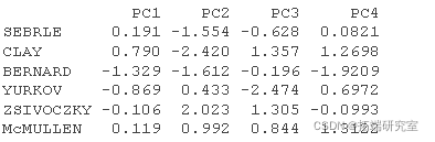
PCA results

• ind.coord = res.pca$x
• Personal Cos2. Two steps:
• Calculate the square distance between each individual and the center of gravity of PCA: d2 = [(var1\_ind\_i - mean\_var1)/sd\_var1]^2 +... + [(var10\_ind\_i - mean\_var10)/sd\_var10]^2 +... +
• Calculate cos2 as ind.coord^2/d2
• Individual contribution to principal components: 100 (1 / number \ _of \ _individuals) (ind.coord ^ 2 / comp_sdev ^ 2). Note that the sum of all contributions per column is 100

#Personal coordinates
#::::::::::::::::::::::::::::::::::
inod <- rpa$x
head(in.c\[, 1:4\])

#Personal Cos2
#:::::::::::::::::::::::::::::::::
# 1.Individual and#Square of distance between center of gravity of PCA
#Square of PCA center of gravity
ceer<- center
scle<- scale

d <- apply(decaive,1,gnce, center, scale)
# 2. Calculate cos2. The sum of each row is 1
is2 <- apply(inrd, 2, cs2, d2)
head(is2\[, 1:4\])

#Personal contribution
#:::::::::::::::::::::::::::::::

inib <- t(apply(iord, 1, conib, 
                       sdev, nrow))
head(inib\[, 1:4\])

Most popular insights

1.matlab partial least squares regression (PLSR) and principal component regression (PCR) And principal component regression (PCR) ")

2.Dimension reduction and visual analysis of principal component pca and t-SNE algorithms for high-dimensional data in R language

3.Basic principle of principal component analysis (PCA) and analysis examples Basic principles and analysis examples ")

4.LASSO regression analysis based on R language

5.Using LASSO regression to predict stock return data analysis

6.lasso regression, ridge ridge regression and elastic net model in r language

7.Partial least squares regression PLS Da data analysis in r language

8.Partial least squares pls regression algorithm in r language

9.R language linear discriminant analysis (LDA), quadratic discriminant analysis (QDA) and canonical discriminant analysis (RDA)