1, Types and tools of date and time data
The modules about date, time and calendar data in Python are datatime, time and calendar
**The data types in the datatime module are as follows: from datatime import*****
| data | Use the Gregorian calendar to store calendar dates (year, month, day) |
|---|---|
| time | Store time as hours, minutes, seconds, microseconds |
| datatime | Store date and time |
| timedelta | Represents the difference between two datatime values (such as day, second, microsecond) |
| tzinfo | The basic type used to store time zone information |
datatime formatting details (compatible with ISO C89)
| %Y | Four digit year |
|---|---|
| %y | Two digit year |
| %m | Two digit months [01, 12] |
| %d | Two digit date number [01, 31] |
| %H | Hour, 24-hour system [00, 23] |
| %I | Hour, 12 hour system [01, 12] |
| %M | Two minutes [00, 59] |
| %S | Seconds [00, 61] (60, 61 are leap seconds) |
| %w | Week date [0 (Sunday), 6] |
| %U | Number of weeks in a year [00, 53]. Take Sunday as the first day of the week, and the date before the first week of the year as' week 0 ' |
| %W | Number of weeks in a year [00, 53]. Monday is the first day of the week, and the date before the first Monday of the year is regarded as' week 0 ' |
| %z | UTC time zone offset in the format of + HHMM or - HHMM; Null if there is no time zone |
| %F | %Abbreviation of Y-%m-%d (e.g., 2021-6-24) |
| %D | %Abbreviation for m/%d/%y (e.g., 06 / 24 / 21) |
datatime object locale specific date formatting options
| %a | Abbreviated working day name |
|---|---|
| %A | Full write workday name |
| %b | Abbreviated month name |
| %B | Full month name |
| %c | Full date and time (e.g. 'Tue 01 May 2012 04:20:57 PM') |
| %p | Regional equivalent of AM or PM |
| %x | Format date suitable for the region (for example, '05 / 01 / 2012' in the United States is May 1) |
| %X | Time appropriate for the region (e.g. '04:24:12 PM') |
import numpy as np
import pandas as pd
np.random.seed(12345)
import matplotlib.pyplot as plt
plt.rc('figure', figsize=(10, 6))
PREVIOUS_MAX_ROWS = pd.options.display.max_rows
pd.options.display.max_rows = 20
np.set_printoptions(precision=4, suppress=True)
from datetime import datetime
now = datetime.now()
now

'''datetime.datetime(2021, 6, 24, 16, 47, 28, 879956)'''

now.year, now.month, now.day

'''(2021, 6, 24)'''

# timedelta represents the time difference between two datetime objects
delta = datetime(2011, 1, 7) - datetime(2008, 6, 24, 8, 15)
delta

'''datetime.timedelta(days=926, seconds=56700)'''

delta.days

'''926'''

delta.seconds

'''56700'''

# Add / subtract a timedelta for the datetime object to generate a new datatime object
from datetime import timedelta
start = datetime(2011, 1, 7)
start + timedelta(12)

'''datetime.datetime(2011, 1, 19, 0, 0)'''

start - 2 * timedelta(12)

'''datetime.datetime(2010, 12, 14, 0, 0)'''
Conversion between string and datatime
# Use the str method or pass a specified format to the strftime method to format the datetime object and the Timestamp object of pandas
stamp = datetime(2011, 1, 3)
str(stamp)

''''2011-01-03 00:00:00''''

stamp.strftime('%Y-%m-%d')

''''2011-01-03''''

# Use datetime Strptime () and format code convert a string to a date
# datetime.strptime() is a good way to convert dates when the format is known
value = '2011-01-03'
datetime.strptime(value, '%Y-%m-%d')

'''datetime.datetime(2011, 1, 3, 0, 0)'''

datestrs = ['7/6/2011', '8/6/2011']
[datetime.strptime(x, '%m/%d/%Y') for x in datestrs]

'''[datetime.datetime(2011, 7, 6, 0, 0), datetime.datetime(2011, 8, 6, 0, 0)]'''

# For the common date format, you can use the parser.xml of the dateutil package Parse method
# dateutil can parse most human understandable date representations
from dateutil.parser import parse
parse('2011-01-03')

'''datetime.datetime(2011, 1, 3, 0, 0)'''

parse('Jan 31, 1997 10:45 PM')

'''datetime.datetime(1997, 1, 31, 22, 45)'''

# Pass dayfirst=True to parse the data whose date is before the month
parse('6/12/2011', dayfirst=True)

'''datetime.datetime(2011, 12, 6, 0, 0)'''

# pd.to_datetime() can convert many different date formats
datestrs = ['2011-07-06 12:00:00', '2011-08-06 00:00:00']
pd.to_datetime(datestrs)

'''DatetimeIndex(['2011-07-06 12:00:00', '2011-08-06 00:00:00'], dtype='datetime64[ns]', freq=None)'''

# pd.to_datetime() can also handle values that are considered missing values (None, empty strings, etc.)
idx = pd.to_datetime(datestrs + [None])
idx

'''DatetimeIndex(['2011-07-06 12:00:00', '2011-08-06 00:00:00', 'NaT'], dtype='datetime64[ns]', freq=None)'''

idx[2]  # NaT(Not a time) is a value where the timestamp data value in pandas is null

'''NaT'''

pd.isnull(idx)

'''array([False, False,  True])'''
2, Time series basis
The basic time Series type in pandas is Series indexed by timestamp;
pandas is usually represented as a python string or datatime object
from datetime import datetime
dates = [datetime(2011, 1, 2), datetime(2011, 1, 5),
         datetime(2011, 1, 7), datetime(2011, 1, 8),
         datetime(2011, 1, 10), datetime(2011, 1, 12)]

# Basic time series in pandas: Series indexed by timestamp
ts = pd.Series(np.random.randn(6), index=dates)
ts

'''
2011-01-02   -0.204708
2011-01-05    0.478943
2011-01-07   -0.519439
2011-01-08   -0.555730
2011-01-10    1.965781
2011-01-12    1.393406
dtype: float64
'''

# These datetime objects are actually placed in a DatetimeIndex
ts.index

'''
DatetimeIndex(['2011-01-02', '2011-01-05', '2011-01-07', '2011-01-08',
               '2011-01-10', '2011-01-12'],
              dtype='datetime64[ns]', freq=None)
'''
# Like other Series, arithmetic operations between time Series with different indexes are automatically aligned by date
ts + ts[::2]

'''
2011-01-02   -0.409415
2011-01-05         NaN
2011-01-07   -1.038877
2011-01-08         NaN
2011-01-10    3.931561
2011-01-12         NaN
dtype: float64
'''

# pandas uses NumPy's datetime64 data type to store timestamps in nanoseconds ns
ts.index.dtype

'''dtype('<M8[ns]')'''

# Each scalar value in DatetimeIndex is the Timestamp object of pandas
stamp = ts.index[0]
stamp

'''Timestamp('2011-01-02 00:00:00')'''
Index, select, subset
# When indexing and selecting based on tags, time series and other pandas Series similar
stamp = ts.index[2]
ts[stamp]

'''-0.5194387150567381'''

# Pass a string that can be interpreted as a date, '20110110' is also OK
ts['1/10/2011']

'''1.9657805725027142'''
# For long time series, you can pass a string selection data that can be interpreted as a year or year month
longer_ts = pd.Series(np.random.randn(1000),
                      index=pd.date_range('1/1/2000', periods=1000))
longer_ts

'''
2000-01-01    0.092908
2000-01-02    0.281746
2000-01-03    0.769023
2000-01-04    1.246435
2000-01-05    1.007189
                ...
2002-09-22    0.930944
2002-09-23   -0.811676
2002-09-24   -1.830156
2002-09-25   -0.138730
2002-09-26    0.334088
Freq: D, Length: 1000, dtype: float64
'''

longer_ts['2001']

'''
2001-01-01    1.599534
2001-01-02    0.474071
2001-01-03    0.151326
2001-01-04   -0.542173
2001-01-05   -0.475496
                ...
2001-12-27    0.057874
2001-12-28   -0.433739
2001-12-29    0.092698
2001-12-30   -1.397820
2001-12-31    1.457823
Freq: D, Length: 365, dtype: float64
'''

longer_ts['2001-05']

'''
2001-05-01   -0.622547
2001-05-02    0.936289
2001-05-03    0.750018
2001-05-04   -0.056715
2001-05-05    2.300675
                ...
2001-05-27    0.235477
2001-05-28    0.111835
2001-05-29   -1.251504
2001-05-30   -2.949343
2001-05-31    0.634634
Freq: D, Length: 31, dtype: float64
'''
ts

'''
2011-01-02   -0.204708
2011-01-05    0.478943
2011-01-07   -0.519439
2011-01-08   -0.555730
2011-01-10    1.965781
2011-01-12    1.393406
dtype: float64
'''

# Pass datatime object for slicing
ts[datetime(2011, 1, 7):]

'''
2011-01-07   -0.519439
2011-01-08   -0.555730
2011-01-10    1.965781
2011-01-12    1.393406
dtype: float64
'''

# Pass timestamps that are not included in the time series for slicing to perform a range query
ts['1/6/2011':'1/11/2011']

'''
2011-01-07   -0.519439
2011-01-08   -0.555730
2011-01-10    1.965781
dtype: float64
'''
Passing a string that can not be interpreted as a date, a datatime object, or a timestamp for slicing are views that produce the original time series; That is, no data is copied, and the changes on the slice will be reflected on the original data
# The equivalent instance method truncate can slice Series between two dates
ts.truncate(before='1/5/2011', after='1/10/2011')

'''
2011-01-05    0.478943
2011-01-07   -0.519439
2011-01-08   -0.555730
2011-01-10    1.965781
dtype: float64
'''
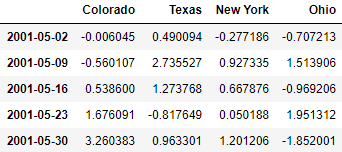
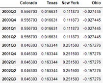
# The above operations also apply to DataFrame
dates = pd.date_range('1/1/2000', periods=100, freq='W-WED')
long_df = pd.DataFrame(np.random.randn(100, 4),
                       index=dates,
                       columns=['Colorado', 'Texas',
                                'New York', 'Ohio'])
long_df.loc['5-2001']
Time series with duplicate indexes
# There are multiple data observations on a timestamp, that is, the time series contains duplicate indexes
dates = pd.DatetimeIndex(['1/1/2000', '1/2/2000', '1/2/2000',
                          '1/2/2000', '1/3/2000'])
dup_ts = pd.Series(np.arange(5), index=dates)
dup_ts

'''
2000-01-01    0
2000-01-02    1
2000-01-02    2
2000-01-02    3
2000-01-03    4
dtype: int32
'''

# Through index is_ Unique property to check whether the index is unique
dup_ts.index.is_unique

'''False'''
# When time Series with duplicate indexes are indexed, whether the result is scalar or Series slice depends on whether the timestamp is repeated
dup_ts['1/3/2000']  # not duplicated

'''4'''

dup_ts['1/2/2000']  # duplicated

'''
2000-01-02    1
2000-01-02    2
2000-01-02    3
dtype: int32
'''
# Aggregate data with duplicate indexes and pass level=0 to groupby
grouped = dup_ts.groupby(level=0)
grouped.mean()

'''
2000-01-01    0
2000-01-02    2
2000-01-03    4
dtype: int32
'''

grouped.count()

'''
2000-01-01    1
2000-01-02    3
2000-01-03    1
dtype: int64
'''
3, Date range, frequency and shift
Generation date range
# pd.date_range(): generate DatatimeIndex of specified length according to specific frequency
# The daily timestamp is generated by default
index = pd.date_range('2012-04-01', '2012-06-01')
index

'''
DatetimeIndex(['2012-04-01', '2012-04-02', '2012-04-03', '2012-04-04',
               '2012-04-05', '2012-04-06', '2012-04-07', '2012-04-08',
               '2012-04-09', '2012-04-10', '2012-04-11', '2012-04-12',
               '2012-04-13', '2012-04-14', '2012-04-15', '2012-04-16',
               '2012-04-17', '2012-04-18', '2012-04-19', '2012-04-20',
               '2012-04-21', '2012-04-22', '2012-04-23', '2012-04-24',
               '2012-04-25', '2012-04-26', '2012-04-27', '2012-04-28',
               '2012-04-29', '2012-04-30', '2012-05-01', '2012-05-02',
               '2012-05-03', '2012-05-04', '2012-05-05', '2012-05-06',
               '2012-05-07', '2012-05-08', '2012-05-09', '2012-05-10',
               '2012-05-11', '2012-05-12', '2012-05-13', '2012-05-14',
               '2012-05-15', '2012-05-16', '2012-05-17', '2012-05-18',
               '2012-05-19', '2012-05-20', '2012-05-21', '2012-05-22',
               '2012-05-23', '2012-05-24', '2012-05-25', '2012-05-26',
               '2012-05-27', '2012-05-28', '2012-05-29', '2012-05-30',
               '2012-05-31', '2012-06-01'],
              dtype='datetime64[ns]', freq='D')
'''
# If you pass only a start or end date, you must pass a number for the generation range to periods
pd.date_range(start='2012-04-01', periods=20)

'''
DatetimeIndex(['2012-04-01', '2012-04-02', '2012-04-03', '2012-04-04',
               '2012-04-05', '2012-04-06', '2012-04-07', '2012-04-08',
               '2012-04-09', '2012-04-10', '2012-04-11', '2012-04-12',
               '2012-04-13', '2012-04-14', '2012-04-15', '2012-04-16',
               '2012-04-17', '2012-04-18', '2012-04-19', '2012-04-20'],
              dtype='datetime64[ns]', freq='D')
'''

pd.date_range(end='2012-06-01', periods=20)

'''
DatetimeIndex(['2012-05-13', '2012-05-14', '2012-05-15', '2012-05-16',
               '2012-05-17', '2012-05-18', '2012-05-19', '2012-05-20',
               '2012-05-21', '2012-05-22', '2012-05-23', '2012-05-24',
               '2012-05-25', '2012-05-26', '2012-05-27', '2012-05-28',
               '2012-05-29', '2012-05-30', '2012-05-31', '2012-06-01'],
              dtype='datetime64[ns]', freq='D')
'''
# Passing the time series frequency to freq will generate DatatimeIndex falling within the specified date range
pd.date_range('2000-01-01', '2000-12-01', freq='BM')

'''
DatetimeIndex(['2000-01-31', '2000-02-29', '2000-03-31', '2000-04-28',
               '2000-05-31', '2000-06-30', '2000-07-31', '2000-08-31',
               '2000-09-29', '2000-10-31', '2000-11-30'],
              dtype='datetime64[ns]', freq='BM')
'''
# pd.date_range() retains the start or end timestamp by default
# Passing normalize=True normalizes the timestamp to zero, that is, the time in the timestamp is removed
pd.date_range('2012-05-02 12:56:31', periods=5)

'''
DatetimeIndex(['2012-05-02 12:56:31', '2012-05-03 12:56:31',
               '2012-05-04 12:56:31', '2012-05-05 12:56:31',
               '2012-05-06 12:56:31'],
              dtype='datetime64[ns]', freq='D')
'''

pd.date_range('2012-05-02 12:56:31', periods=5, normalize=True)

'''
DatetimeIndex(['2012-05-02', '2012-05-03', '2012-05-04', '2012-05-05',
               '2012-05-06'],
              dtype='datetime64[ns]', freq='D')
'''
| Base time series frequency | ||
|---|---|---|
| alias | Offset type | describe |
| D | Day | Day of calendar day |
| M | BusinessDay | Every day of the working day |
| H | Hour | Per hour |
| T or min | Minute | per minute |
| S | Second | Per second |
| L or ms | Milli | Per millisecond (1 / 1000 second) |
| U | Micro | Per microsecond (1 / 1000000 second) |
| M | MonthEnd | Last day of the calendar month |
| BM | BusinessMonthEnd | Last day of the month on the working day |
| MS | MonthBegin | First day of the calendar month |
| BMS | BusinessMonthBegin | First day of the month on the working day |
| W-MON,W-TUE,...... | Week | According to the given day of the week, take the day of the week (MON,TUE,WED,THU,FRI,SAT or SUN) |
| WOM-1MON,WOM-2MON,...... | WeekOfMonth | Create week separated dates on the first / second / third or fourth week of the month (e.g. WOM-3FRI: the third Friday of each month) |
| Q-JAN,Q-FEB,...... | QuarterEnd | The quarterly date of the last calendar day of each month to indicate the year in which the month ends (JAN,FEB,MAR,APR,MAY,JUN,JUL,AUG,SEP,OCT,NOV or DEC) |
| BQ-JAN,BQ-FEB,...... | BusinessQuarterEnd | The quarterly date corresponding to the last working day of each month to represent the year when the month ends |
| QS-JAN,QS-FEB,...... | QuarterBegin | The quarterly date corresponding to the first calendar day of each month to indicate the year when the month ends |
| BQS-JAN,BQS-FEB,...... | BusinessQuarterBegin | The quarterly date corresponding to the first working day of each month to represent the year in which the month ends |
| A-JAN,A-FEB,...... | YearEnd | The annual date (JAN,FEB,MAR,APR,MAY,JUN,JUL,AUG,SEP,OCT,NOV or DEC) of the last calendar day of the month in which the given month is located |
| BA-JAN,BA-FEB,...... | BusinessYearEnd | The annual date of the last working day of the month in which the given month is located |
| AS-JAN,AS-FEB,...... | YearBegin | The annual date of the first calendar day of the month in which the given month is located |
| BAS-JAN,BAS-FEB,...... | BusinessYearBegin | The annual date of the first working day of the month in which the given month is located |
Frequency and date offset
# For each base frequency, there is an object that can be used to define the date offset
# For example, the frequency per Hour can be represented by the Hour class
from pandas.tseries.offsets import Hour, Minute
hour = Hour()
hour

'''<Hour>'''

# Pass an integer to define a multiple of the offset
four_hours = Hour(4)
four_hours

'''<4 * Hours>'''

pd.date_range('2000-01-01', '2000-01-03 23:59', freq='4h')

'''
DatetimeIndex(['2000-01-01 00:00:00', '2000-01-01 04:00:00',
               '2000-01-01 08:00:00', '2000-01-01 12:00:00',
               '2000-01-01 16:00:00', '2000-01-01 20:00:00',
               '2000-01-02 00:00:00', '2000-01-02 04:00:00',
               '2000-01-02 08:00:00', '2000-01-02 12:00:00',
               '2000-01-02 16:00:00', '2000-01-02 20:00:00',
               '2000-01-03 00:00:00', '2000-01-03 04:00:00',
               '2000-01-03 08:00:00', '2000-01-03 12:00:00',
               '2000-01-03 16:00:00', '2000-01-03 20:00:00'],
              dtype='datetime64[ns]', freq='4H')
'''

# Multiple offsets can be combined by addition
Hour(2) + Minute(30)

'''<150 * Minutes>'''

pd.date_range('2000-01-01', periods=10, freq='1h30min')

'''
DatetimeIndex(['2000-01-01 00:00:00', '2000-01-01 01:30:00',
               '2000-01-01 03:00:00', '2000-01-01 04:30:00',
               '2000-01-01 06:00:00', '2000-01-01 07:30:00',
               '2000-01-01 09:00:00', '2000-01-01 10:30:00',
               '2000-01-01 12:00:00', '2000-01-01 13:30:00'],
              dtype='datetime64[ns]', freq='90T')
'''

# Pass freq='WOM-3FRI 'to get the date of the third Friday of a week in the specified date range
rng = pd.date_range('2012-01-01', '2012-09-01', freq='WOM-3FRI')
list(rng)

'''
[Timestamp('2012-01-20 00:00:00', freq='WOM-3FRI'),
 Timestamp('2012-02-17 00:00:00', freq='WOM-3FRI'),
 Timestamp('2012-03-16 00:00:00', freq='WOM-3FRI'),
 Timestamp('2012-04-20 00:00:00', freq='WOM-3FRI'),
 Timestamp('2012-05-18 00:00:00', freq='WOM-3FRI'),
 Timestamp('2012-06-15 00:00:00', freq='WOM-3FRI'),
 Timestamp('2012-07-20 00:00:00', freq='WOM-3FRI'),
 Timestamp('2012-08-17 00:00:00', freq='WOM-3FRI')]
'''
Shift date forward or backward
# Shift refers to moving the data in the time series forward or backward in time
# It is implemented through the shift() method of Series or DataFrame
ts = pd.Series(np.random.randn(4),
               index=pd.date_range('1/1/2000', periods=4, freq='M'))
ts

'''
2000-01-31   -0.066748
2000-02-29    0.838639
2000-03-31   -0.117388
2000-04-30   -0.517795
Freq: M, dtype: float64
'''

# Shifting data forward introduces a missing value in the start bit
ts.shift(2)

'''
2000-01-31         NaN
2000-02-29         NaN
2000-03-31   -0.066748
2000-04-30    0.838639
Freq: M, dtype: float64
'''

# Shifting data backward will introduce missing values at the end
ts.shift(-2)

'''
2000-01-31   -0.117388
2000-02-29   -0.517795
2000-03-31         NaN
2000-04-30         NaN
Freq: M, dtype: float64
'''
shift() is often used to calculate the percentage change of time series or DataFrame multi column time series, i.e. ts/ts.shift(1)-1
# Passing the frequency freq='M 'to shift will shift the timestamp instead of the data
# Here, it means that the timestamp is shifted forward by two months, i.e. + 2 months
# Note the difference between the forward shift of data and the forward shift of timestamp
ts.shift(2, freq='M')

'''
2000-03-31   -0.066748
2000-04-30    0.838639
2000-05-31   -0.117388
2000-06-30   -0.517795
Freq: M, dtype: float64
'''

# Passing freq='D 'means that each timestamp is shifted forward by 3 days, i.e. + 3 days
ts.shift(3, freq='D')

'''
2000-02-03   -0.066748
2000-03-03    0.838639
2000-04-03   -0.117388
2000-05-03   -0.517795
dtype: float64
'''

# # Passing freq='90T 'means that each timestamp is shifted forward by 90 minutes
ts.shift(1, freq='90T')

'''
2000-01-31 01:30:00   -0.066748
2000-02-29 01:30:00    0.838639
2000-03-31 01:30:00   -0.117388
2000-04-30 01:30:00   -0.517795
dtype: float64
'''
Shift date using offset
# pandas date offset can also be done using datatime or Timestamp objects
from pandas.tseries.offsets import Day, MonthEnd
now = datetime(2011, 11, 17)
now + 3 * Day()

'''Timestamp('2011-11-20 00:00:00')'''

# Anchor offset, such as MonthEnd, and BusinessMonthEnd will roll forward the date to the next date
now + MonthEnd()

'''Timestamp('2011-11-30 00:00:00')'''

now + MonthEnd(2)

'''Timestamp('2011-12-31 00:00:00')'''

# The anchor offset can be used to scroll the date forward or backward displayed by rollforward and rollback
offset = MonthEnd()
offset.rollforward(now)

'''Timestamp('2011-11-30 00:00:00')'''

offset.rollback(now)

'''Timestamp('2011-12-31 00:00:00')'''
# Use the shift method with groupby
ts = pd.Series(np.random.randn(20),
               index=pd.date_range('1/15/2000', periods=20, freq='4d'))
ts

'''
2000-01-15   -0.116696
2000-01-19    2.389645
2000-01-23   -0.932454
2000-01-27   -0.229331
2000-01-31   -1.140330
2000-02-04    0.439920
2000-02-08   -0.823758
2000-02-12   -0.520930
2000-02-16    0.350282
2000-02-20    0.204395
2000-02-24    0.133445
2000-02-28    0.327905
2000-03-03    0.072153
2000-03-07    0.131678
2000-03-11   -1.297459
2000-03-15    0.997747
2000-03-19    0.870955
2000-03-23   -0.991253
2000-03-27    0.151699
2000-03-31    1.266151
Freq: 4D, dtype: float64
'''

# offset.rollforward will operate on the timestamp index of ts by default
ts.groupby(offset.rollforward).mean()

'''
2000-01-31   -0.005833
2000-02-29    0.015894
2000-03-31    0.150209
dtype: float64
'''

# The resample() method can achieve the same effect
ts.resample('M').mean()

'''
2000-01-31   -0.005833
2000-02-29    0.015894
2000-03-31    0.150209
Freq: M, dtype: float64
'''
4, Time zone processing
# The time zone is usually represented as the offset of UTC. The time zone information comes from a third-party library pytz
import pytz
pytz.common_timezones[-5:]

'''['US/Eastern', 'US/Hawaii', 'US/Mountain', 'US/Pacific', 'UTC']'''

# pytz.timezone() gets pytz's time zone object
tz = pytz.timezone('America/New_York')
tz

'''<DstTzInfo 'America/New_York' LMT-1 day, 19:04:00 STD>'''
Localization and conversion of time zones
rng = pd.date_range('3/9/2012 9:30', periods=6, freq='D')
ts = pd.Series(np.random.randn(len(rng)), index=rng)
ts

'''
2012-03-09 09:30:00   -0.202469
2012-03-10 09:30:00    0.050718
2012-03-11 09:30:00    0.639869
2012-03-12 09:30:00    0.597594
2012-03-13 09:30:00   -0.797246
2012-03-14 09:30:00    0.472879
Freq: D, dtype: float64
'''

# Used to return the time zone
print(ts.index.tz)

'''None'''

# Date ranges can be generated from time zone collections
pd.date_range('3/9/2012 9:30', periods=10, freq='D', tz='UTC')

'''
DatetimeIndex(['2012-03-09 09:30:00+00:00', '2012-03-10 09:30:00+00:00',
               '2012-03-11 09:30:00+00:00', '2012-03-12 09:30:00+00:00',
               '2012-03-13 09:30:00+00:00', '2012-03-14 09:30:00+00:00',
               '2012-03-15 09:30:00+00:00', '2012-03-16 09:30:00+00:00',
               '2012-03-17 09:30:00+00:00', '2012-03-18 09:30:00+00:00'],
              dtype='datetime64[ns, UTC]', freq='D')
'''
ts

'''
2012-03-09 09:30:00   -0.202469
2012-03-10 09:30:00    0.050718
2012-03-11 09:30:00    0.639869
2012-03-12 09:30:00    0.597594
2012-03-13 09:30:00   -0.797246
2012-03-14 09:30:00    0.472879
Freq: D, dtype: float64
'''

# With tz_localize() converts a simple time zone to a localized time zone
ts_utc = ts.tz_localize('UTC')
ts_utc

'''
2012-03-09 09:30:00+00:00   -0.202469
2012-03-10 09:30:00+00:00    0.050718
2012-03-11 09:30:00+00:00    0.639869
2012-03-12 09:30:00+00:00    0.597594
2012-03-13 09:30:00+00:00   -0.797246
2012-03-14 09:30:00+00:00    0.472879
Freq: D, dtype: float64
'''

ts_utc.index

'''
DatetimeIndex(['2012-03-09 09:30:00+00:00', '2012-03-10 09:30:00+00:00',
               '2012-03-11 09:30:00+00:00', '2012-03-12 09:30:00+00:00',
               '2012-03-13 09:30:00+00:00', '2012-03-14 09:30:00+00:00'],
              dtype='datetime64[ns, UTC]', freq='D')
'''

# Localized time zones are available through tz_convert() to another time zone
ts_utc.tz_convert('America/New_York')

'''
2012-03-09 04:30:00-05:00   -0.202469
2012-03-10 04:30:00-05:00    0.050718
2012-03-11 05:30:00-04:00    0.639869
2012-03-12 05:30:00-04:00    0.597594
2012-03-13 05:30:00-04:00   -0.797246
2012-03-14 05:30:00-04:00    0.472879
Freq: D, dtype: float64
'''

# With tz_localize() localizes the time zone to the New York time zone
ts_eastern = ts.tz_localize('America/New_York')
ts_eastern.tz_convert('UTC')

'''
2012-03-09 14:30:00+00:00   -0.202469
2012-03-10 14:30:00+00:00    0.050718
2012-03-11 13:30:00+00:00    0.639869
2012-03-12 13:30:00+00:00    0.597594
2012-03-13 13:30:00+00:00   -0.797246
2012-03-14 13:30:00+00:00    0.472879
dtype: float64
'''

ts_eastern.tz_convert('Europe/Berlin')

'''
2012-03-09 15:30:00+01:00   -0.202469
2012-03-10 15:30:00+01:00    0.050718
2012-03-11 14:30:00+01:00    0.639869
2012-03-12 14:30:00+01:00    0.597594
2012-03-13 14:30:00+01:00   -0.797246
2012-03-14 14:30:00+01:00    0.472879
dtype: float64
'''

# tz_localize(),tz_convert() is also an instance method of DatetimeIndex
ts.index.tz_localize('Asia/Shanghai')

'''
DatetimeIndex(['2012-03-09 09:30:00+08:00', '2012-03-10 09:30:00+08:00',
               '2012-03-11 09:30:00+08:00', '2012-03-12 09:30:00+08:00',
               '2012-03-13 09:30:00+08:00', '2012-03-14 09:30:00+08:00'],
              dtype='datetime64[ns, Asia/Shanghai]', freq=None)
'''
Operation of time zone aware timestamp object
# Separate Timestamp objects can also be localized to time zone aware timestamps and time zone conversion
stamp = pd.Timestamp('2011-03-12 04:00')
stamp_utc = stamp.tz_localize('utc')
stamp_utc.tz_convert('America/New_York')

'''Timestamp('2011-03-11 23:00:00-0500', tz='America/New_York')'''

# Pass time zone when creating Timestamp object
stamp_moscow = pd.Timestamp('2011-03-12 04:00', tz='Europe/Moscow')
stamp_moscow

'''Timestamp('2011-03-12 04:00:00+0300', tz='Europe/Moscow')'''

# The time zone aware Timestamp object stores UTC Timestamp values in nanoseconds since the Unix era (1970-1-1)
stamp_utc.value

'''1299902400000000000'''

# The number of nanoseconds UTC timestamp value is unchanged in time zone conversion
stamp_utc.tz_convert('America/New_York').value

'''1299902400000000000'''
from pandas.tseries.offsets import Hour
stamp = pd.Timestamp('2012-03-12 01:30', tz='US/Eastern')
stamp

'''Timestamp('2012-03-12 01:30:00-0400', tz='US/Eastern')'''

# Hour() added is 1 hour of UTC
stamp + Hour()

'''Timestamp('2012-03-12 02:30:00-0400', tz='US/Eastern')'''

stamp = pd.Timestamp('2012-11-04 00:30', tz='US/Eastern')
stamp

'''Timestamp('2012-11-04 00:30:00-0400', tz='US/Eastern')'''

stamp + 2 * Hour()

'''Timestamp('2012-11-04 01:30:00-0500', tz='US/Eastern')'''
Operation in different time intervals
# Operations in different time intervals will be automatically converted to UTC time first, and the result is also UTC time
rng = pd.date_range('3/7/2012 9:30', periods=10, freq='B')
ts = pd.Series(np.random.randn(len(rng)), index=rng)
ts

'''
2012-03-07 09:30:00    0.522356
2012-03-08 09:30:00   -0.546348
2012-03-09 09:30:00   -0.733537
2012-03-12 09:30:00    1.302736
2012-03-13 09:30:00    0.022199
2012-03-14 09:30:00    0.364287
2012-03-15 09:30:00   -0.922839
2012-03-16 09:30:00    0.312656
2012-03-19 09:30:00   -1.128497
2012-03-20 09:30:00   -0.333488
Freq: B, dtype: float64
'''

ts1 = ts[:7].tz_localize('Europe/London')
ts2 = ts1[2:].tz_convert('Europe/Moscow')
result = ts1 + ts2
result.index

'''
DatetimeIndex(['2012-03-07 09:30:00+00:00', '2012-03-08 09:30:00+00:00',
               '2012-03-09 09:30:00+00:00', '2012-03-12 09:30:00+00:00',
               '2012-03-13 09:30:00+00:00', '2012-03-14 09:30:00+00:00',
               '2012-03-15 09:30:00+00:00'],
              dtype='datetime64[ns, UTC]', freq=None)
'''
5, Time interval and interval arithmetic
The Period class represents a time interval, that is, a time range. For example, some days, some months, some quarters, some years
# The following Period objects represent the Period from January 1, 2007 to December 31, 2007
p = pd.Period(2007, freq='A-DEC')
p

'''Period('2007', 'A-DEC')'''

# When doing addition and subtraction, shift directly according to the frequency freq='A-DEC '
p + 5

'''Period('2012', 'A-DEC')'''

p - 2

'''Period('2005', 'A-DEC')'''

# The difference between two intervals with the same frequency is a multiple of the frequency
pd.Period('2014', freq='A-DEC') - p

'''<7 * YearEnds: month=12>'''
# Use PD period_ Range() can construct regular interval sequences
rng = pd.period_range('2000-01-01', '2000-06-30', freq='M')
rng

'''PeriodIndex(['2000-01', '2000-02', '2000-03', '2000-04', '2000-05', '2000-06'], dtype='period[M]', freq='M')'''

# PeriodIndex class stores interval sequence, which can be used as axis index of pandas data structure
pd.Series(np.random.randn(6), index=rng)

'''
2000-01   -0.514551
2000-02   -0.559782
2000-03   -0.783408
2000-04   -1.797685
2000-05   -0.172670
2000-06    0.680215
Freq: M, dtype: float64
'''
# pd.PeriodIndex() generates the PeriodIndex class
values = ['2001Q3', '2002Q2', '2003Q1']
index = pd.PeriodIndex(values, freq='Q-DEC')
index

'''PeriodIndex(['2001Q3', '2002Q2', '2003Q1'], dtype='period[Q-DEC]', freq='Q-DEC')'''
Interval frequency conversion
# Create a Period interval with December as the end month of the year
p = pd.Period('2007', freq='A-DEC')
p

'''Period('2007', 'A-DEC')'''

# asfreq() can convert interval and PeriodIndex objects to other frequencies
p.asfreq('M', how='start')

'''Period('2007-01', 'M')'''

p.asfreq('M', how='end')

'''Period('2007-12', 'M')'''
# Create a Period interval with June as the end month of the year
# In this case, the period from July 2006 to June 2007 is regarded as the year of 2007
p = pd.Period('2007', freq='A-JUN')
p

'''Period('2007', 'A-JUN')'''

# Specifying how as' start 'will return the first month of 2007
# Since June is the end month of the year, the first month is 2006-07
p.asfreq('M', 'start')

'''Period('2006-07', 'M')'''

p.asfreq('M', 'end')

'''Period('2007-06', 'M')'''
# The above is the conversion from low frequency to high frequency, or from high frequency to low frequency, that is, similar month to year
p = pd.Period('Aug-2007', 'M')
p.asfreq('A-JUN')
# When 'A-JUN' is imported, the end month of the table name year is June, so 2007-8 belongs to 2008

'''Period('2008', 'A-JUN')'''

p = pd.Period('Aug-2007', 'M')
p.asfreq('A-SEP')
# When 'A-SEP' is imported, the end month of the table name year is June, so 2007-8 belongs to 2007

'''Period('2007', 'A-SEP')'''
# The complete PeriodIndex object or time series can do the above similar conversion
rng = pd.period_range('2006', '2009', freq='A-DEC')
ts = pd.Series(np.random.randn(len(rng)), index=rng)
ts

'''
2006    1.607578
2007    0.200381
2008   -0.834068
2009   -0.302988
Freq: A-DEC, dtype: float64
'''

ts.asfreq('M', how='start')

'''
2006-01    1.607578
2007-01    0.200381
2008-01   -0.834068
2009-01   -0.302988
Freq: M, dtype: float64
'''

ts.asfreq('B', how='end')

'''
2006-12-29    1.607578
2007-12-31    0.200381
2008-12-31   -0.834068
2009-12-31   -0.302988
Freq: B, dtype: float64
'''
Quarterly interval frequency
# Quarterly data are generally at the end of the fiscal year, so similar to 2012Q4 generally have different meanings
# Set freq='Q-JAN ', indicating that the month at the end of the quarter is January
# Therefore, 2012Q4 refers to the four months from November 2011 to January 2012
p = pd.Period('2012Q4', freq='Q-JAN')
p

'''Period('2012Q4', 'Q-JAN')'''

p.asfreq('D', 'start')

'''Period('2011-11-01', 'D')'''

p.asfreq('D', 'end')

'''Period('2012-01-31', 'D')'''

# Get the timestamp of 4:00 p.m. on the penultimate business day of the quarter
# p. Asfreq ('b ',' e ') - 1 get the penultimate work of the quarter
# (p.asfreq('B', 'e') - 1). Asfreq ('t ','s') converts the obtained date into minutes and is the zero point of the day
# Another '+ 16 * 60' is the number of minutes plus 4 p.m
p4pm = (p.asfreq('B', 'e') - 1).asfreq('T', 's') + 16 * 60
p4pm

'''Period('2012-01-30 16:00', 'T')'''

# Use to_timestamp() to timestamp
p4pm.to_timestamp()

'''Timestamp('2012-01-30 16:00:00')'''
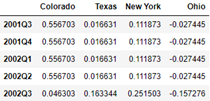
# pd.period_range() is used to generate quarterly series
rng = pd.period_range('2011Q3', '2012Q4', freq='Q-JAN')
ts = pd.Series(np.arange(len(rng)), index=rng)
ts

'''
2011Q3    0
2011Q4    1
2012Q1    2
2012Q2    3
2012Q3    4
2012Q4    5
Freq: Q-JAN, dtype: int32
'''

# Get the timestamp of 4:00 p.m. on the penultimate business day of the quarter
new_rng = (rng.asfreq('B', 'e') - 1).asfreq('T', 's') + 16 * 60
ts.index = new_rng.to_timestamp()
ts

'''
2010-10-28 16:00:00    0
2011-01-28 16:00:00    1
2011-04-28 16:00:00    2
2011-07-28 16:00:00    3
2011-10-28 16:00:00    4
2012-01-30 16:00:00    5
dtype: int32
'''
Convert timestamp to interval (and inverse conversion)
rng = pd.date_range('2000-01-01', periods=3, freq='M')
ts = pd.Series(np.random.randn(3), index=rng)
ts

'''
2000-01-31    1.663261
2000-02-29   -0.996206
2000-03-31    1.521760
Freq: M, dtype: float64
'''

# Series and DataFrame indexed by timestamp are available to_ The period() method is converted to an interval
pts = ts.to_period()
pts

'''
2000-01    1.663261
2000-02   -0.996206
2000-03    1.521760
Freq: M, dtype: float64
'''
rng = pd.date_range('1/29/2000', periods=6, freq='D')
ts2 = pd.Series(np.random.randn(6), index=rng)
ts2

'''
2000-01-29    0.244175
2000-01-30    0.423331
2000-01-31   -0.654040
2000-02-01    2.089154
2000-02-02   -0.060220
2000-02-03   -0.167933
Freq: D, dtype: float64
'''

# After interval conversion, it is allowed that the index contains repeated intervals
ts2.to_period('M')

'''
2000-01    0.244175
2000-01    0.423331
2000-01   -0.654040
2000-02    2.089154
2000-02   -0.060220
2000-02   -0.167933
Freq: M, dtype: float64
'''
# Create JAN-1 as the month at the end of the last quarter of each year
rng = pd.period_range('2011Q3', '2012Q4', freq='Q-JAN')
ts3 = pd.Series(np.arange(len(rng)), index=rng)
ts3

'''
2011Q3    0
2011Q4    1
2012Q1    2
2012Q2    3
2012Q3    4
2012Q4    5
Freq: Q-JAN, dtype: int32
'''

# to_timestamp() converts the interval to a timestamp
# how defaults to start, and takes the zero point of the first month of the quarter as the index; how='end 'can also be set
ts3.to_timestamp()

'''
2010-08-01    0
2010-11-01    1
2011-02-01    2
2011-05-01    3
2011-08-01    4
2011-11-01    5
Freq: QS-NOV, dtype: int32
'''
Generate PeriodIndex from array
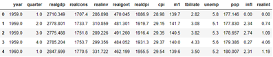
data = pd.read_csv('examples/macrodata.csv')
data.head(5)
data.year.head()
'''
0 1959.0
1 1959.0
2 1959.0
3 1959.0
4 1960.0
Name: year, dtype: float64
'''
data.quarter.head()
'''
0 1.0
1 2.0
2 3.0
3 4.0
4 1.0
Name: quarter, dtype: float64
'''
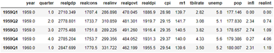
index = pd.PeriodIndex(year=data.year, quarter=data.quarter,
freq='Q-DEC')
index
'''
PeriodIndex(['1959Q1', '1959Q2', '1959Q3', '1959Q4', '1960Q1', '1960Q2',
'1960Q3', '1960Q4', '1961Q1', '1961Q2',
...
'2007Q2', '2007Q3', '2007Q4', '2008Q1', '2008Q2', '2008Q3',
'2008Q4', '2009Q1', '2009Q2', '2009Q3'],
dtype='period[Q-DEC]', length=203, freq='Q-DEC')
'''
data.index = index
data.head()
6, Resampling and frequency conversion
Resampling: the process of converting a time series from one frequency to another
Down sampling: aggregates higher frequencies to lower frequencies
Up sampling: converts low frequencies to high frequencies
However, not all resampling are the above two types, such as converting W-WED to W-REI
The resample() method of the pandas object performs frequency conversion, which has a function similar to group by
rng = pd.date_range('2000-01-01', periods=100, freq='D')
ts = pd.Series(np.random.randn(len(rng)), index=rng)
ts

'''
2000-01-01    0.631634
2000-01-02   -1.594313
2000-01-03   -1.519937
2000-01-04    1.108752
2000-01-05    1.255853
                ...
2000-04-05   -0.423776
2000-04-06    0.789740
2000-04-07    0.937568
2000-04-08   -2.253294
2000-04-09   -1.772919
Freq: D, Length: 100, dtype: float64
'''

ts.resample('M').mean()

'''
2000-01-31   -0.165893
2000-02-29    0.078606
2000-03-31    0.223811
2000-04-30   -0.063643
Freq: M, dtype: float64
'''

# kind='period 'specifies that the type of index in the result is period
ts.resample('M', kind='period').mean()

'''
2000-01   -0.165893
2000-02    0.078606
2000-03    0.223811
2000-04   -0.063643
Freq: M, dtype: float64
'''
| Parameters of the resample() method | |
|---|---|
| freq | Sampling frequency, which is a string or DataOffset object (such as' 5min ','M', or Second(1)) |
| axis | Which axis to sample along, the default axis=0 |
| fill_method | The difference method when sampling upward. Interpolation is not allowed by default. Options include 'fill' and 'bfill' |
| closed | In down sampling, which segment of each interval is closed can be 'right' or 'left' |
| label | In downward sampling, mark the aggregation results with the box label of 'right' /'left '(for example, the 5-minute interval from 9:30 to 9:35 can be marked as 9:30 / 9:35) |
| loffset | Adjust the time of the box label (for example, '1s' / Second(-1) can move the aggregate label forward for 1 second) |
| limit | When filling forward or backward, the maximum value of the filling interval |
| kind | Specify that the index in the result is interval ('period ') or timestamp ('timestamp'), and the default is time series index |
| convention | When resampling an interval, the convention used to convert a low-frequency period to a high-frequency period is' start 'by default and' end 'is optional |
Down sampling
Things to consider when using resample() to sample down:
- Which side of each interval is closed
- How to mark each aggregated box at the beginning or end of the interval
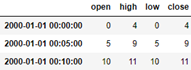
rng = pd.date_range('2000-01-01', periods=12, freq='T')
ts = pd.Series(np.arange(12), index=rng)
ts

'''
2000-01-01 00:00:00     0
2000-01-01 00:01:00     1
2000-01-01 00:02:00     2
2000-01-01 00:03:00     3
2000-01-01 00:04:00     4
2000-01-01 00:05:00     5
2000-01-01 00:06:00     6
2000-01-01 00:07:00     7
2000-01-01 00:08:00     8
2000-01-01 00:09:00     9
2000-01-01 00:10:00    10
2000-01-01 00:11:00    11
Freq: T, dtype: int32
'''

# The default is closed='left ', which divides the index interval into [00:00,00:05], [00:05,00:10),
# Then aggregate the data at such intervals
# By default, label='left ', the left side of the index interval is taken as the row label in the result
ts.resample('5min', closed='left').sum()

'''
2000-01-01 00:00:00    10
2000-01-01 00:05:00    35
2000-01-01 00:10:00    21
Freq: 5T, dtype: int32
'''

ts.resample('5min', closed='right').sum()

'''
1999-12-31 23:55:00     0
2000-01-01 00:00:00    15
2000-01-01 00:05:00    40
2000-01-01 00:10:00    11
Freq: 5T, dtype: int32
'''

ts.resample('5min', closed='right', label='right').sum()

'''
2000-01-01 00:00:00     0
2000-01-01 00:05:00    15
2000-01-01 00:10:00    40
2000-01-01 00:15:00    11
Freq: 5T, dtype: int32
'''

# Setting loffset='1s' will move the index in the result to the right for 1 second, that is, add 1 second
ts.resample('5min', closed='right',
            label='right', loffset='1s').sum()

'''
2000-01-01 00:00:01     0
2000-01-01 00:05:01    15
2000-01-01 00:10:01    40
2000-01-01 00:15:01    11
Freq: 5T, dtype: int32
'''
Start peak valley end (OHLC) resampling
# ohlc() gets the first value, the last value, the maximum value, and the minimum value within the index interval
ts.resample('5min').ohlc()
Up sampling and difference
# When upsampling, aggregation is not required, and asfreq() is used for frequency conversion
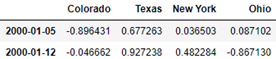
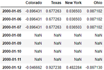
frame = pd.DataFrame(np.random.randn(2, 4),
index=pd.date_range('1/1/2000', periods=2,
freq='W-WED'),
columns=['Colorado', 'Texas', 'New York', 'Ohio'])
frame
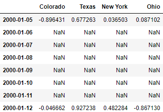
# When asfreq() is used for frequency conversion, missing values will be introduced when converting from low frequency to high frequency
df_daily = frame.resample('D').asfreq()
df_daily
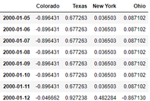
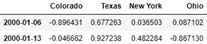
# If you do not want to introduce the missing value, you can set the filling value with fill()
frame.resample('D').ffill()
# If limit=2 is passed to fill(), only two rows of data will be filled forward
frame.resample('D').ffill(limit=2)
frame.resample('W-THU').ffill()
Resampling with Periods
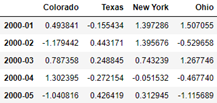
frame = pd.DataFrame(np.random.randn(24, 4),
                     index=pd.period_range('1-2000', '12-2001',
                                           freq='M'),
                     columns=['Colorado', 'Texas', 'New York', 'Ohio'])
frame[:5]
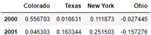
# Downward sampling, frequency 'A-DEC', year, December as the last month at the end of the year
annual_frame = frame.resample('A-DEC').mean()
annual_frame
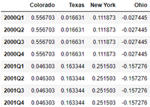
# Sample upward and set the fill method fill(), with the default convention='start '
# Q-DEC: quarter, December is the last month of the last quarter
annual_frame.resample('Q-DEC').ffill()
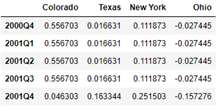
# Sample upward and set the filling method fill()
# Pass convention='end ', set the index in the result to start at the end of the quarter of the original first index year and end at the end of the quarter of the original last index year
annual_frame.resample('Q-DEC', convention='end').ffill()
In down sampling, the frequency in the original sequence must be the sub interval of the frequency in the result; Month year
When sampling upward, the frequency in the original sequence must be the parent interval of the frequency in the result; Year month
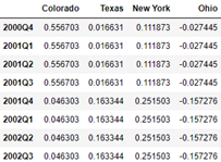
Carefully figure out the following operations and understand them through drawing
annual_frame.resample('Q-MAR').ffill()
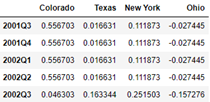
annual_frame.resample('Q-MAR', convention='end').ffill()
annual_frame.resample('Q-APR').ffill()
annual_frame.resample('Q-APR', convention='end').ffill()
7, Move window function
Like other statistical functions, the moving window function will automatically exclude missing data
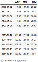
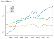
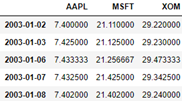
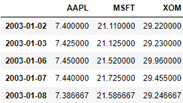
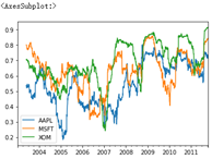
close_px_all = pd.read_csv('examples/stock_px_2.csv',
                           parse_dates=True, index_col=0)
close_px = close_px_all[['AAPL', 'MSFT', 'XOM']]
close_px
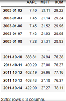
# Resampling according to working day frequency
close_px = close_px.resample('B').ffill()
close_px
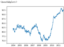
%matplotlib inline
close_px.AAPL.plot()
# rolling() can be called through a window (i.e. the number 250 passed in below) on Series and DataFrame
# Here is the grouping according to 250 sliding windows
close_px.AAPL.rolling(250).mean().plot()
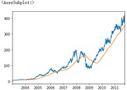
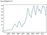
# Transfer min_ If periods = 10, the standard deviation of the first 10 closed transactions will be calculated first, then the standard deviation of the first 11 transactions, and so on
# Until the first 250 groups of data are calculated, the moving window is used to calculate the standard deviation
appl_std250 = close_px.AAPL.rolling(250, min_periods=10).std()
appl_std250[5:12]

'''
2003-01-09         NaN
2003-01-10         NaN
2003-01-13         NaN
2003-01-14         NaN
2003-01-15    0.077496
2003-01-16    0.074760
2003-01-17    0.112368
Freq: B, Name: AAPL, dtype: float64
'''

appl_std250.plot()
# expanding() will make the window expand gradually. The left side will not move and the right side will expand to the right; Find the mean value of the extended window
# For example, here, 2003-01-16 is the average of the original 01-16 and 01-15
# For example, here, 2003-01-17 is the average value of the original 01-15 to 01-17
expanding_mean = appl_std250.expanding().mean()
expanding_mean[5:12]

'''
2003-01-09         NaN
2003-01-10         NaN
2003-01-13         NaN
2003-01-14         NaN
2003-01-15    0.077496
2003-01-16    0.076128
2003-01-17    0.088208
Freq: B, Name: AAPL, dtype: float64
'''

# Pass log = true and take the logarithm of y
close_px.rolling(60).mean().plot(logy=True)
# Pass' 20D ', fixed to 20 days of the calendar day for moving; In the previous pass, 250 days of the index column is taken as a window
close_px.rolling('20D').mean().head()
# Pass' 3D ', fixed to take the 3 days of the calendar day for moving average
# Therefore, the mean value of 2003-01-06 in the results remains unchanged because there are no data on No. 4 and No. 5
close_px.rolling('3D').mean().head()
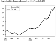
Exponential weighting function
# Specify the attenuation factor through span=30, that is, the weights are 2 / 31, 2 / 31 * 29 / 31
aapl_px = close_px.AAPL['2006':'2007']
# Simple moving average
ma60 = aapl_px.rolling(30, min_periods=20).mean()
# Exponential weighted average
ewma60 = aapl_px.ewm(span=30).mean()
ma60.plot(style='k--', label='Simple MA')
ewma60.plot(style='k-', label='EW MA')
plt.legend()
Binary moving window function
Operate two time series at the same time, using the same moving window size, such as corr() or covariance
spx_px = close_px_all['SPX']
spx_rets = spx_px.pct_change()
spx_rets

'''
2003-01-02         NaN
2003-01-03   -0.000484
2003-01-06    0.022474
2003-01-07   -0.006545
2003-01-08   -0.014086
                ...
2011-10-10    0.034125
2011-10-11    0.000544
2011-10-12    0.009795
2011-10-13   -0.002974
2011-10-14    0.017380
Name: SPX, Length: 2214, dtype: float64
'''

returns = close_px.pct_change()
returns
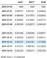
# Notice here, returns AAPL has 2292 rows of data, while spx_rets has 2214 rows of data
# Therefore, their row indexes are not exactly the same when calculating mobile windows
# Under normal circumstances, this will not happen. It may be the author's mistake
# corr() calculates the rolling correlation coefficient
corr = returns.AAPL.rolling(125, min_periods=100).corr(spx_rets)
corr.plot()
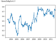
corr = returns.rolling(125, min_periods=100).corr(spx_rets)
corr.plot()
User defined moving window function
# Using apply() on rolling() and related methods can use custom array functions in the moving window
from scipy.stats import percentileofscore
# What percentage of samples x is less than 0.02
score_at_2percent = lambda x: percentileofscore(x, 0.02)
result = returns.AAPL.rolling(250).apply(score_at_2percent)
result.plot()