Introduction to machine learning for programmers (IV) - common skills in the training process
This article will focus on some common skills in machine learning training using pytorch. Mastering them can make you get twice the result with half the effort.
Most of the codes used will be based on the last example in the previous article, that is, predicting wages according to code farming conditions 🙀, If you didn't read the last article, please click here see.
Save and read model status
In pytorch, all operations are based on the tensor object, and the parameters of the model are also tensor. If we save the trained tensor to the hard disk and then read it from the hard disk next time, we can use it directly.
Let's take a look at how to save a single tensor. The following code runs in python REPL:
# Reference pytorch
>>> import torch

# Create a new tensor object
>>> a = torch.tensor([1, 2, 3], dtype=torch.float)

# Save tensor to file 1 pt
>>> torch.save(a, "1.pt")

# From file 1 PT read tensor
>>> b = torch.load("1.pt")
>>> b
tensor([1., 2., 3.])
torch. When saving tensor, python's pickle format will be used. This format ensures compatibility between different python versions, but does not support compressed content. Therefore, if tensor is very large, the saved file will occupy a lot of space. We can compress it before saving and decompress it before reading to reduce the file size:
# Reference compression library
>>> import gzip

# Save tensor to file 1 Pt, gzip compression is used when saving
>>> torch.save(a, gzip.GzipFile("1.pt.gz", "wb"))

# From file 1 PT reads tensor, and gzip is used for decompression when reading
>>> b = torch.load(gzip.GzipFile("1.pt.gz", "rb"))
>>> b
tensor([1., 2., 3.])
torch.save not only supports saving a single tensor object, but also supports saving the tensor list or dictionary (in fact, it can also save python objects other than tensor, as long as the pickle format supports it). We can call {state_dict # get a set containing all the parameters of the model, and then torch Save can save the state of the model:
>>> from torch import nn
>>> class MyModel(nn.Module):
...     def __init__(self):
...         super().__init__()
...         self.layer1 = nn.Linear(in_features=8, out_features=100)
...         self.layer2 = nn.Linear(in_features=100, out_features=50)
...         self.layer3 = nn.Linear(in_features=50, out_features=1)
...     def forward(self, x):
...         hidden1 = nn.functional.relu(self.layer1(x))
...         hidden2 = nn.functional.relu(self.layer2(hidden1))
...         y = self.layer3(hidden2)
...         return y
...
>>> model = MyModel()
>>> model.state_dict()
OrderedDict([('layer1.weight', tensor([[ 0.2261,  0.2008,  0.0833, -0.2020, -0.0674,  0.2717, -0.0076,  0.1984],
        Omit en route output
          0.1347,  0.1356]])), ('layer3.bias', tensor([0.0769]))])

>>> torch.save(model.state_dict(), gzip.GzipFile("model.pt.gz", "wb"))
To read the model status, you can use load_state_dict} function, but you need to ensure that the parameter definition of the model does not change, otherwise the reading will make an error:
>>> new_model = MyModel()
>>> new_model.load_state_dict(torch.load(gzip.GzipFile("model.pt.gz", "rb")))
<All keys matched successfully>
A very important detail is that if you read the model state instead of preparing to continue training, but used to predict other data, you should call the eval function to prohibit automatic differentiation and other functions, which can speed up the operation speed:
>>> new_model.eval()
pytorch supports not only saving and reading the model state, but also saving and reading the whole model, including code and parameters. However, I do not recommend this method, because the model definition will not be seen when using, and the class libraries or functions dependent on the model will not be saved together. Therefore, you still have to load them in advance, otherwise errors will occur:
>>> torch.save(model, gzip.GzipFile("model.pt.gz", "wb"))
>>> new_model = torch.load(gzip.GzipFile("model.pt.gz", "rb"))
Record the change of accuracy of training set and verification set
We can record the changes in the accuracy of the training set and the verification set during the training process to observe whether it can converge, how fast the training is, and whether fitting problems have occurred. The following is a code example:
# Reference pytorch and pandas and the matchlib used to display the chart
import pandas
import torch
from torch import nn
from matplotlib import pyplot

# Define model
class MyModel(nn.Module):
    def __init__(self):
        super().__init__()
        self.layer1 = nn.Linear(in_features=8, out_features=100)
        self.layer2 = nn.Linear(in_features=100, out_features=50)
        self.layer3 = nn.Linear(in_features=50, out_features=1)

    def forward(self, x):
        hidden1 = nn.functional.relu(self.layer1(x))
        hidden2 = nn.functional.relu(self.layer2(hidden1))
        y = self.layer3(hidden2)
        return y

# Assign an initial value to the random number generator so that each run can generate the same random number
# This is to make the training process repeatable, or you can choose not to do so
torch.random.manual_seed(0)

# Create model instance
model = MyModel()

# Create loss calculator
loss_function = torch.nn.MSELoss()

# Create parameter adjuster
optimizer = torch.optim.SGD(model.parameters(), lr=0.0000001)

# Read raw dataset from csv
df = pandas.read_csv('salary.csv')
dataset_tensor = torch.tensor(df.values, dtype=torch.float)

# Segmentation training set (60%), verification set (20%) and test set (20%)
random_indices = torch.randperm(dataset_tensor.shape[0])
traning_indices = random_indices[:int(len(random_indices)*0.6)]
validating_indices = random_indices[int(len(random_indices)*0.6):int(len(random_indices)*0.8):]
testing_indices = random_indices[int(len(random_indices)*0.8):]
traning_set_x = dataset_tensor[traning_indices][:,:-1]
traning_set_y = dataset_tensor[traning_indices][:,-1:]
validating_set_x = dataset_tensor[validating_indices][:,:-1]
validating_set_y = dataset_tensor[validating_indices][:,-1:]
testing_set_x = dataset_tensor[testing_indices][:,:-1]
testing_set_y = dataset_tensor[testing_indices][:,-1:]

# Record the change of accuracy of training set and verification set
traning_accuracy_history = []
validating_accuracy_history = []

# Start the training process
for epoch in range(1, 500):
    print(f"epoch: {epoch}")

    # Train and modify the parameters according to the training set
    # Switching the model to training mode will enable automatic differentiation, batchnorm and Dropout
    model.train()

    traning_accuracy_list = []
    for batch in range(0, traning_set_x.shape[0], 100):
        # Divide batches and only calculate 100 groups of data at a time
        batch_x = traning_set_x[batch:batch+100]
        batch_y = traning_set_y[batch:batch+100]
        # Calculate predicted value
        predicted = model(batch_x)
        # Calculate loss
        loss = loss_function(predicted, batch_y)
        # Deriving function value from loss automatic differentiation
        loss.backward()
        # Use the parameter adjuster to adjust the parameters
        optimizer.step()
        # Clear leading function value
        optimizer.zero_grad()
        # Record the accuracy of this batch, torch no_ Grad stands for temporarily disabling the automatic differentiation function
        with torch.no_grad():
            traning_accuracy_list.append(1 - ((batch_y - predicted).abs() / batch_y).mean().item())
    traning_accuracy = sum(traning_accuracy_list) / len(traning_accuracy_list)
    traning_accuracy_history.append(traning_accuracy)
    print(f"training accuracy: {traning_accuracy}")

    # Check validation set
    # Switching the model to validation mode will disable automatic differentiation, batchnorm and Dropout
    model.eval()
    predicted = model(validating_set_x)
    validating_accuracy = 1 - ((validating_set_y - predicted).abs() / validating_set_y).mean()
    validating_accuracy_history.append(validating_accuracy.item())
    print(f"validating x: {validating_set_x}, y: {validating_set_y}, predicted: {predicted}")
    print(f"validating accuracy: {validating_accuracy}")

# Check test set
predicted = model(testing_set_x)
testing_accuracy = 1 - ((testing_set_y - predicted).abs() / testing_set_y).mean()
print(f"testing x: {testing_set_x}, y: {testing_set_y}, predicted: {predicted}")
print(f"testing accuracy: {testing_accuracy}")

# Display the correct rate change of training set and verification set
pyplot.plot(traning_accuracy_history, label="traning")
pyplot.plot(validating_accuracy_history, label="validing")
pyplot.ylim(0, 1)
pyplot.legend()
pyplot.show()

# Manual input data prediction output
while True:
    try:
        print("enter input:")
        r = list(map(float, input().split(",")))
        x = torch.tensor(r).view(1, len(r))
        print(model(x)[0,0].item())
    except Exception as e:
        print("error:", e)
After 500 rounds of training, the following chart will be generated:
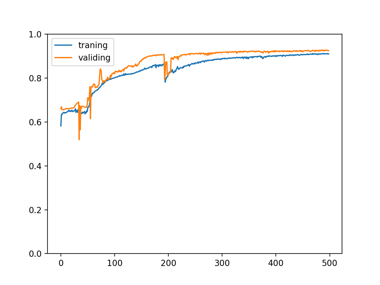
We can see from the chart that the accuracy of the training set and the verification set gradually increases with the training, and the two accuracy rates are very close, which means that the training is very successful. The model has mastered the law for the training set and can successfully predict the untrained verification set, but in fact, it is difficult for us to see such a chart, This is because the data set in the example is carefully constructed and generates enough data.
We may also see the following types of charts representing different situations:
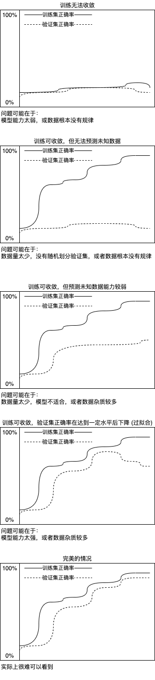
If there is enough data, the data follows a certain law and has less impurities, the training set and verification set are evenly distributed, and an appropriate model is used, the ideal situation can be achieved, but it is difficult to do in practice 😩. By analyzing the changes in the accuracy of the training set and the verification set, we can locate where the problem occurs. The over fitting problem can be solved by early stopping (mentioned in the first article). Next, let's see how to decide when to stop training.
Decide when to stop training
Remember the training process mentioned in the first article? We will learn how to implement this training process in Code:
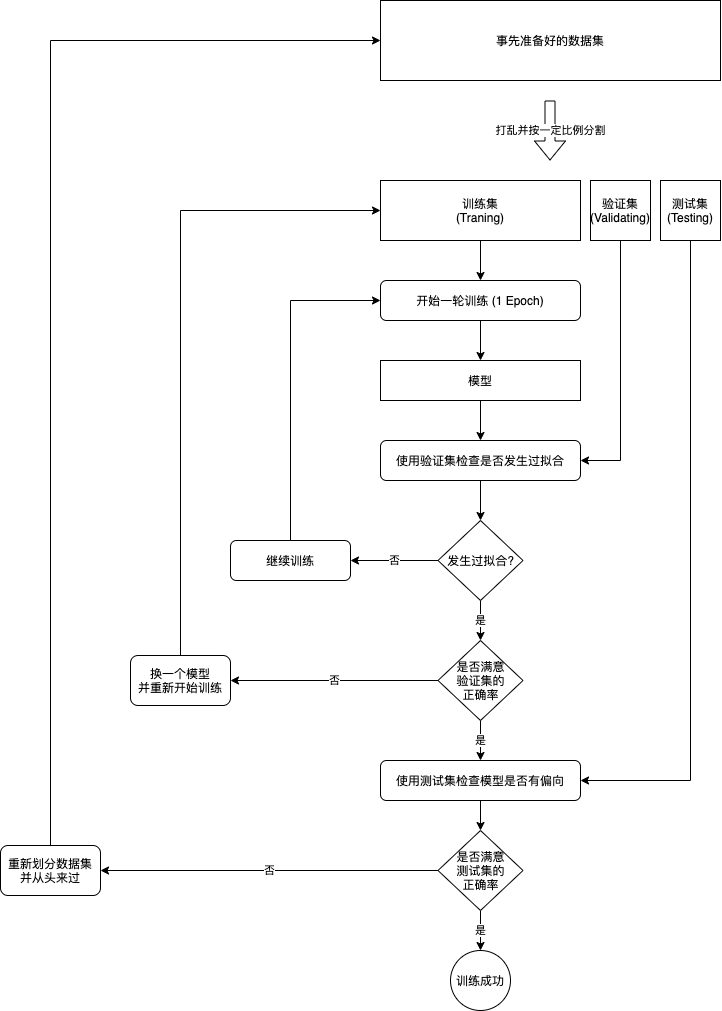
To judge whether fitting has occurred, you can simply record the highest accuracy rate of the verification set in history. If the highest accuracy rate is not refreshed after many times of training, the training will be ended. While recording the highest accuracy, we also need to save the state of the model. At this time, the model has found enough laws, but the parameters have not been modified to adapt to the impurities in the training set. It can achieve the best effect to predict the unknown data. This technique, also known as early stopping, is a very common technique in machine learning.
The code implementation is as follows:
# Reference pytorch and pandas and the matchlib used to display the chart
import pandas
import torch
from torch import nn
from matplotlib import pyplot

# Define model
class MyModel(nn.Module):
    def __init__(self):
        super().__init__()
        self.layer1 = nn.Linear(in_features=8, out_features=100)
        self.layer2 = nn.Linear(in_features=100, out_features=50)
        self.layer3 = nn.Linear(in_features=50, out_features=1)

    def forward(self, x):
        hidden1 = nn.functional.relu(self.layer1(x))
        hidden2 = nn.functional.relu(self.layer2(hidden1))
        y = self.layer3(hidden2)
        return y

# Assign an initial value to the random number generator so that each run can generate the same random number
# This is to make the training process repeatable, or you can choose not to do so
torch.random.manual_seed(0)

# Create model instance
model = MyModel()

# Create loss calculator
loss_function = torch.nn.MSELoss()

# Create parameter adjuster
optimizer = torch.optim.SGD(model.parameters(), lr=0.0000001)

# Read raw dataset from csv
df = pandas.read_csv('salary.csv')
dataset_tensor = torch.tensor(df.values, dtype=torch.float)

# Segmentation training set (60%), verification set (20%) and test set (20%)
random_indices = torch.randperm(dataset_tensor.shape[0])
traning_indices = random_indices[:int(len(random_indices)*0.6)]
validating_indices = random_indices[int(len(random_indices)*0.6):int(len(random_indices)*0.8):]
testing_indices = random_indices[int(len(random_indices)*0.8):]
traning_set_x = dataset_tensor[traning_indices][:,:-1]
traning_set_y = dataset_tensor[traning_indices][:,-1:]
validating_set_x = dataset_tensor[validating_indices][:,:-1]
validating_set_y = dataset_tensor[validating_indices][:,-1:]
testing_set_x = dataset_tensor[testing_indices][:,:-1]
testing_set_y = dataset_tensor[testing_indices][:,-1:]

# Record the change of accuracy of training set and verification set
traning_accuracy_history = []
validating_accuracy_history = []

# Record the highest validation set accuracy
validating_accuracy_highest = 0
validating_accuracy_highest_epoch = 0

# Start the training process
for epoch in range(1, 10000):
    print(f"epoch: {epoch}")

    # Train and modify the parameters according to the training set
    # Switching the model to training mode will enable automatic differentiation, batchnorm and Dropout
    model.train()

    traning_accuracy_list = []
    for batch in range(0, traning_set_x.shape[0], 100):
        # Divide batches and only calculate 100 groups of data at a time
        batch_x = traning_set_x[batch:batch+100]
        batch_y = traning_set_y[batch:batch+100]
        # Calculate predicted value
        predicted = model(batch_x)
        # Calculate loss
        loss = loss_function(predicted, batch_y)
        # Deriving function value from loss automatic differentiation
        loss.backward()
        # Use the parameter adjuster to adjust the parameters
        optimizer.step()
        # Clear leading function value
        optimizer.zero_grad()
        # Record the accuracy of this batch, torch no_ Grad stands for temporarily disabling the automatic differentiation function
        with torch.no_grad():
            traning_accuracy_list.append(1 - ((batch_y - predicted).abs() / batch_y).mean().item())
    traning_accuracy = sum(traning_accuracy_list) / len(traning_accuracy_list)
    traning_accuracy_history.append(traning_accuracy)
    print(f"training accuracy: {traning_accuracy}")

    # Check validation set
    # Switching the model to validation mode will disable automatic differentiation, batchnorm and Dropout
    model.eval()
    predicted = model(validating_set_x)
    validating_accuracy = 1 - ((validating_set_y - predicted).abs() / validating_set_y).mean()
    validating_accuracy_history.append(validating_accuracy.item())
    print(f"validating x: {validating_set_x}, y: {validating_set_y}, predicted: {predicted}")
    print(f"validating accuracy: {validating_accuracy}")

    # Record the highest accuracy of the verification set and the current model state, and judge whether the record is still not refreshed after 100 training
    if validating_accuracy > validating_accuracy_highest:
        validating_accuracy_highest = validating_accuracy
        validating_accuracy_highest_epoch = epoch
        torch.save(model.state_dict(), "model.pt")
        print("highest validating accuracy updated")
    elif epoch - validating_accuracy_highest_epoch > 100:
        # After 100 times of training, you still didn't refresh the record and ended the training
        print("stop training because highest validating accuracy not updated in 100 epoches")
        break

# Use the model state at the highest accuracy
print(f"highest validating accuracy: {validating_accuracy_highest}",
    f"from epoch {validating_accuracy_highest_epoch}")
model.load_state_dict(torch.load("model.pt"))

# Check test set
predicted = model(testing_set_x)
testing_accuracy = 1 - ((testing_set_y - predicted).abs() / testing_set_y).mean()
print(f"testing x: {testing_set_x}, y: {testing_set_y}, predicted: {predicted}")
print(f"testing accuracy: {testing_accuracy}")

# Display the correct rate change of training set and verification set
pyplot.plot(traning_accuracy_history, label="traning")
pyplot.plot(validating_accuracy_history, label="validing")
pyplot.ylim(0, 1)
pyplot.legend()
pyplot.show()

# Manual input data prediction output
while True:
    try:
        print("enter input:")
        r = list(map(float, input().split(",")))
        x = torch.tensor(r).view(1, len(r))
        print(model(x)[0,0].item())
    except Exception as e:
        print("error:", e)
The final output is as follows:
Omit starting output
stop training because highest validating accuracy not updated in 100 epoches
highest validating accuracy: 0.93173748254776 from epoch 645
testing x: tensor([[48., 1., 18., ..., 5., 0., 5.],
[22., 1., 2., ..., 2., 1., 2.],
[24., 0., 1., ..., 3., 2., 0.],
...,
[24., 0., 4., ..., 0., 1., 1.],
[39., 0., 0., ..., 0., 5., 5.],
[36., 0., 5., ..., 3., 0., 3.]]), y: tensor([[14000.],
[10500.],
[13000.],
...,
[15500.],
[12000.],
[19000.]]), predicted: tensor([[15612.1895],
[10705.9873],
[12577.7988],
...,
[16281.9277],
[10780.5996],
[19780.3281]], grad_fn=<AddmmBackward>)
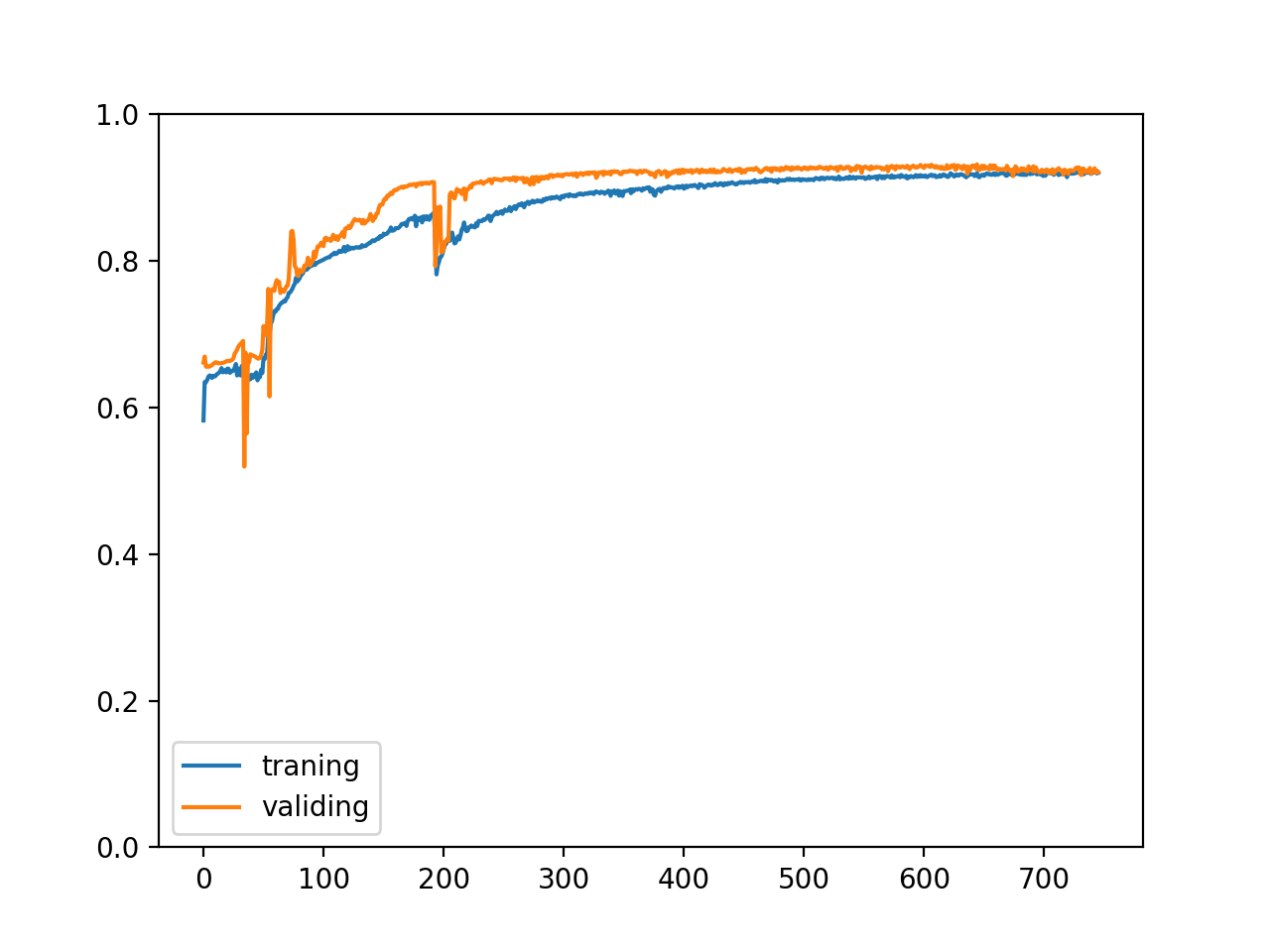
testing accuracy: 0.9330222606658936
The accuracy of the training set and the verification set changes as follows. We can see that we have stopped at a good place 😸, There will be no improvement if you continue training:
Improve program structure
We can also make the following improvements to the program structure:
- Separate the process of preparing data sets and training
- Read data in batches during training
- Provide the interface and use the trained model
So far, the training codes we have seen are written in a program to prepare data sets, train, evaluate and use after training. This is easy to understand, but it will waste time in actual business. If you find that a model is not suitable and need to modify the model, you have to start from scratch. We can separate the process of preparing data sets and training. First read the original data and convert it to the tensor object, then save it to the hard disk, and then read the tensor object from the hard disk for training. In this way, if we need to modify the model but do not need to modify the input and output, we can save the first step.
In the actual business, the data may be very large. It is impossible to read all the data into the memory and divide it into batches. At this time, we can read the original data and convert it to the tensor object in batches, and then read it from the hard disk batch by batch during the training process, so as to prevent the problem of insufficient memory.
Finally, we can provide an external interface to use the trained model. If your program is written in Python, you can call it directly. However, if your program is written in other languages, you may need to establish a python server to provide REST services or use TorchScript for cross language interaction. For details, please refer to the official course.
To sum up, we will split the following processes:
- Read the original dataset and convert it to the tensor object
- Save tensor objects to hard disk in batches
- Read tensor objects from hard disk in batches and train them
- Save the model state to the hard disk during training (generally choose to save the model state with the highest accuracy of the verification set)
- Provide the interface and use the trained model
Here is the improved example code:
import os
import sys
import pandas
import torch
import gzip
import itertools
from torch import nn
from matplotlib import pyplot

class MyModel(nn.Module):
    """A model for predicting wages according to the code farming conditions"""
    def __init__(self):
        super().__init__()
        self.layer1 = nn.Linear(in_features=8, out_features=100)
        self.layer2 = nn.Linear(in_features=100, out_features=50)
        self.layer3 = nn.Linear(in_features=50, out_features=1)

    def forward(self, x):
        hidden1 = nn.functional.relu(self.layer1(x))
        hidden2 = nn.functional.relu(self.layer2(hidden1))
        y = self.layer3(hidden2)
        return y

def save_tensor(tensor, path):
    """preservation tensor Object to file"""
    torch.save(tensor, gzip.GzipFile(path, "wb"))

def load_tensor(path):
    """Read from file tensor object"""
    return torch.load(gzip.GzipFile(path, "rb"))

def prepare():
    """Preparation training"""
    # After the dataset is converted to tensor, it will be saved in the data folder
    if not os.path.isdir("data"):
        os.makedirs("data")

    # Read the original data set from csv, and read 2000 rows each time in batches
    for batch, df in enumerate(pandas.read_csv('salary.csv', chunksize=2000)):
        dataset_tensor = torch.tensor(df.values, dtype=torch.float)

        # Segmentation training set (60%), verification set (20%) and test set (20%)
        random_indices = torch.randperm(dataset_tensor.shape[0])
        traning_indices = random_indices[:int(len(random_indices)*0.6)]
        validating_indices = random_indices[int(len(random_indices)*0.6):int(len(random_indices)*0.8):]
        testing_indices = random_indices[int(len(random_indices)*0.8):]
        training_set = dataset_tensor[traning_indices]
        validating_set = dataset_tensor[validating_indices]
        testing_set = dataset_tensor[testing_indices]

        # Save to hard disk
        save_tensor(training_set, f"data/training_set.{batch}.pt")
        save_tensor(validating_set, f"data/validating_set.{batch}.pt")
        save_tensor(testing_set, f"data/testing_set.{batch}.pt")
        print(f"batch {batch} saved")

def train():
    """Start training"""
    # Create model instance
    model = MyModel()

    # Create loss calculator
    loss_function = torch.nn.MSELoss()

    # Create parameter adjuster
    optimizer = torch.optim.SGD(model.parameters(), lr=0.0000001)

    # Record the change of accuracy of training set and verification set
    traning_accuracy_history = []
    validating_accuracy_history = []

    # Record the highest validation set accuracy
    validating_accuracy_highest = 0
    validating_accuracy_highest_epoch = 0

    # Tool functions for reading batches
    def read_batches(base_path):
        for batch in itertools.count():
            path = f"{base_path}.{batch}.pt"
            if not os.path.isfile(path):
                break
            yield load_tensor(path)

    # Tool function for calculating accuracy
    def calc_accuracy(actual, predicted):
        return max(0, 1 - ((actual - predicted).abs() / actual.abs()).mean().item())

    # Start the training process
    for epoch in range(1, 10000):
        print(f"epoch: {epoch}")

        # Train and modify the parameters according to the training set
        # Switching the model to training mode will enable automatic differentiation, batchnorm and Dropout
        model.train()
        traning_accuracy_list = []
        for batch in read_batches("data/training_set"):
            # Splitting small batches is helpful to generalize the model
             for index in range(0, batch.shape[0], 100):
                # Divide input and output
                batch_x = batch[index:index+100,:-1]
                batch_y = batch[index:index+100,-1:]
                # Calculate predicted value
                predicted = model(batch_x)
                # Calculate loss
                loss = loss_function(predicted, batch_y)
                # Deriving function value from loss automatic differentiation
                loss.backward()
                # Use the parameter adjuster to adjust the parameters
                optimizer.step()
                # Clear leading function value
                optimizer.zero_grad()
                # Record the accuracy of this batch, torch no_ Grad stands for temporarily disabling the automatic differentiation function
                with torch.no_grad():
                    traning_accuracy_list.append(calc_accuracy(batch_y, predicted))
        traning_accuracy = sum(traning_accuracy_list) / len(traning_accuracy_list)
        traning_accuracy_history.append(traning_accuracy)
        print(f"training accuracy: {traning_accuracy}")

        # Check validation set
        # Switching the model to validation mode will disable automatic differentiation, batchnorm and Dropout
        model.eval()
        validating_accuracy_list = []
        for batch in read_batches("data/validating_set"):
            validating_accuracy_list.append(calc_accuracy(batch[:,-1:],  model(batch[:,:-1])))
        validating_accuracy = sum(validating_accuracy_list) / len(validating_accuracy_list)
        validating_accuracy_history.append(validating_accuracy)
        print(f"validating accuracy: {validating_accuracy}")

        # Record the highest accuracy of the verification set and the current model state, and judge whether the record is still not refreshed after 100 training
        if validating_accuracy > validating_accuracy_highest:
            validating_accuracy_highest = validating_accuracy
            validating_accuracy_highest_epoch = epoch
            save_tensor(model.state_dict(), "model.pt")
            print("highest validating accuracy updated")
        elif epoch - validating_accuracy_highest_epoch > 100:
            # After 100 times of training, you still didn't refresh the record and ended the training
            print("stop training because highest validating accuracy not updated in 100 epoches")
            break

    # Use the model state at the highest accuracy
    print(f"highest validating accuracy: {validating_accuracy_highest}",
        f"from epoch {validating_accuracy_highest_epoch}")
    model.load_state_dict(load_tensor("model.pt"))

    # Check test set
    testing_accuracy_list = []
    for batch in read_batches("data/testing_set"):
        testing_accuracy_list.append(calc_accuracy(batch[:,-1:],  model(batch[:,:-1])))
    testing_accuracy = sum(testing_accuracy_list) / len(testing_accuracy_list)
    print(f"testing accuracy: {testing_accuracy}")

    # Display the correct rate change of training set and verification set
    pyplot.plot(traning_accuracy_history, label="traning")
    pyplot.plot(validating_accuracy_history, label="validing")
    pyplot.ylim(0, 1)
    pyplot.legend()
    pyplot.show()

def eval_model():
    """Use the trained model"""
    parameters = [
        "Age",
        "Gender (0: Male, 1: Female)",
        "Years of work experience",
        "Java Skill (0 ~ 5)",
        "NET Skill (0 ~ 5)",
        "JS Skill (0 ~ 5)",
        "CSS Skill (0 ~ 5)",
        "HTML Skill (0 ~ 5)"
    ]

    # Create a model instance, load the trained state, and then switch to verification mode
    model = MyModel()
    model.load_state_dict(load_tensor("model.pt"))
    model.eval()

    # Query input and predict output
    while True:
        try:
            x = torch.tensor([int(input(f"Your {p}: ")) for p in parameters], dtype=torch.float)
            # Conversion to a matrix with one row and one column is not required here, but it is recommended because not all models support non batch input
            x = x.view(1, len(x))
            y = model(x)
            print("Your estimated salary:", y[0,0].item(), "\n")
        except Exception as e:
            print("error:", e)

def main():
    """Main function"""
    if len(sys.argv) < 2:
        print(f"Please run: {sys.argv[0]} prepare|train|eval")
        exit()

    # Assign an initial value to the random number generator so that each run can generate the same random number
    # This is to make the process reproducible, or you can choose not to do so
    torch.random.manual_seed(0)

    # Select the operation according to the command line parameters
    operation = sys.argv[1]
    if operation == "prepare":
        prepare()
    elif operation == "train":
        train()
    elif operation == "eval":
        eval_model()
    else:
        raise ValueError(f"Unsupported operation: {operation}")

if __name__ == "__main__":
    main()
Execute the following commands to go through the whole process. If you need to adjust the model, you can directly re run the train to avoid the time consumption of prepare:
python3 example.py prepare
python3 example.py train
python3 example.py eval
Note that the above codes are different from the previous codes in disrupting data sets and batch processing. The above codes will read csv files in sections, and then disrupt each section and then segment the training set, verification set and test set. This can also ensure that the data is evenly distributed in each set. The accuracy changes of the final training set and verification set are as follows:
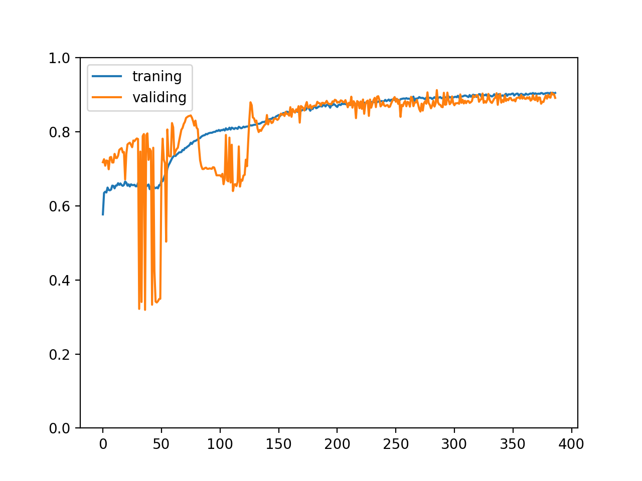
Normalized input and output values
So far, when we train, we directly give the original input value of the model, and then use the original output value to adjust the parameters. The problem is that if the input value is very large, the derivative value will be very large, and if the output value is very large, there will be a lot of times to adjust the parameters, In the past, we used a very, very small learning ratio (0.0000001) to avoid this problem, but there is a better way, that is, normalizing the input and output values. Normalization here refers to scaling the input value and output value in a certain proportion, so that most of the values fall in the range of - 1 ~ 1. In the example of predicting wages according to the code farming conditions, we can multiply the age and years of work experience by 0.01 (range 0 ~ 100 years), various skills by 0.02 (range 0 ~ 5), wages by 0.0001 (in 10000), and set_ Tensor # can be realized by:
# Multiplies each row by the specified factor
dataset_tensor *= torch.tensor([0.01, 1, 0.01, 0.2, 0.2, 0.2, 0.2, 0.2, 0.0001])
Then modify the learning ratio to 0.01:
optimizer = torch.optim.SGD(model.parameters(), lr=0.01)
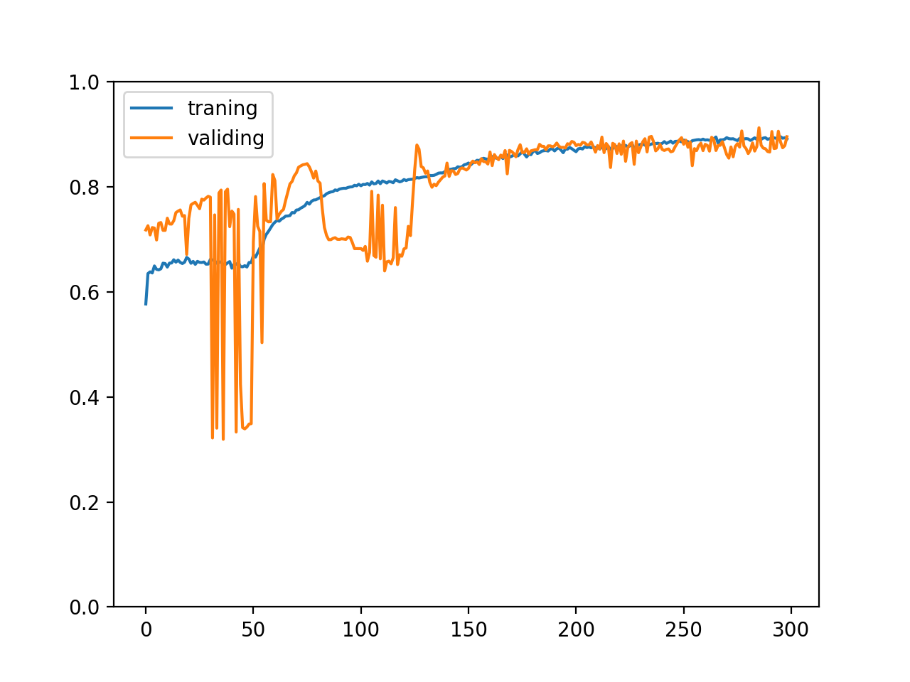
The correct rate of 300 times of comparative training changes as follows:
Before normalizing input and output values
After normalizing input and output values
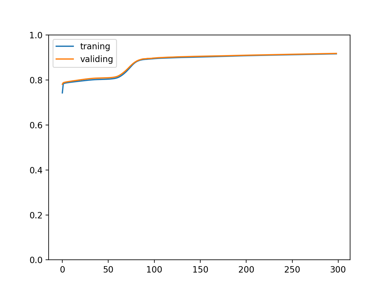
You can see that the effect is quite amazing 😈, After normalizing the input and output values, the training speed becomes faster and the change curve of accuracy is much smoother. In fact, this must be done. If some data sets are not normalized, they cannot learn at all. Allowing the model to receive and output smaller values (- 1 ~ 1 interval) can prevent the explosion of derivation values and use a higher learning ratio to speed up the training speed.
Also, don't forget to scale the input and output values when using the model:
x = torch.tensor([int(input(f"Your {p}: ")) for p in parameters], dtype=torch.float)
x *= torch.tensor([0.01, 1, 0.01, 0.2, 0.2, 0.2, 0.2, 0.2])
# Conversion to a matrix with one row and one column is not required here, but it is recommended because not all models support non batch input
x = x.view(1, len(x))
y = model(x) * 10000
print("Your estimated salary:", y[0,0].item(), "\n")
Use Dropout to help generalize the model
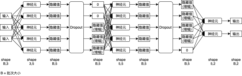
As mentioned in the previous content, if the model capability is too strong or there are many data impurities, the model may adapt to the impurities in the data to achieve a higher accuracy (over fitting phenomenon). At this time, although the accuracy of the training set will increase, the accuracy of the verification set will maintain or even decrease, and the ability of the model to deal with unknown data will decrease. To prevent over fitting and enhance the ability of the model to deal with unknown data, it is also called generalized model. One of the means of generalized model is to use dropout. Dropout will randomly shield some neurons during training, so that the output of these neurons is 0. At the same time, increase the output of unshielded neurons, so that the total output value is close to the original level, The advantage of this is that the model will try to find out how to correctly predict the results (weaken the correlation between cross layer neurons) after some neurons are shielded, and finally lead the model to better grasp the law of data.
The following figure is an example of neural network after using Dropout (3 inputs, 2 outputs, 5 hidden values for each layer of 3 layers):
Next, let's look at how to use Dropout in pytoch:
# Reference pytorch class library
>>> import torch

# Create a Dropout function that masks 20%
>>> dropout = torch.nn.Dropout(0.2)

# Define a tensor (assuming that this tensor is the output of a neural network layer)
>>> a = torch.tensor(range(1, 11), dtype=torch.float)
>>> a
tensor([ 1.,  2.,  3.,  4.,  5.,  6.,  7.,  8.,  9., 10.])

# Apply Dropout function
# We can see that the value without shielding will increase accordingly (divided by 0.8) to keep the total value at the original level
# In addition, the number of shields will fluctuate according to the probability, which is not necessarily 100% equal to the proportion we set (there are 1 value shielded and 3 values shielded here)
>>> dropout(a)
tensor([ 0.0000,  2.5000,  3.7500,  5.0000,  6.2500,  7.5000,  8.7500, 10.0000,
        11.2500, 12.5000])
>>> dropout(a)
tensor([ 1.2500,  2.5000,  3.7500,  5.0000,  6.2500,  7.5000,  8.7500,  0.0000,
        11.2500,  0.0000])
>>> dropout(a)
tensor([ 1.2500,  2.5000,  3.7500,  5.0000,  6.2500,  7.5000,  8.7500,  0.0000,
        11.2500, 12.5000])
>>> dropout(a)
tensor([ 1.2500,  2.5000,  3.7500,  5.0000,  6.2500,  7.5000,  0.0000, 10.0000,
        11.2500,  0.0000])
>>> dropout(a)
tensor([ 1.2500,  2.5000,  3.7500,  5.0000,  0.0000,  7.5000,  8.7500, 10.0000,
        11.2500,  0.0000])
>>> dropout(a)
tensor([ 1.2500,  2.5000,  0.0000,  5.0000,  0.0000,  7.5000,  8.7500, 10.0000,
        11.2500, 12.5000])
>>> dropout(a)
tensor([ 0.0000,  2.5000,  3.7500,  5.0000,  6.2500,  7.5000,  0.0000, 10.0000,
         0.0000,  0.0000])
Next, let's see how to apply Dropout to the model. First, let's reproduce the over fitting phenomenon, increase the number of neurons in the model and reduce the amount of data in the training set:
Code of model part:
class MyModel(nn.Module):
    """A model for predicting wages according to the code farming conditions"""
    def __init__(self):
        super().__init__()
        self.layer1 = nn.Linear(in_features=8, out_features=200)
        self.layer2 = nn.Linear(in_features=200, out_features=100)
        self.layer3 = nn.Linear(in_features=100, out_features=1)

    def forward(self, x):
        hidden1 = nn.functional.relu(self.layer1(x))
        hidden2 = nn.functional.relu(self.layer2(hidden1))
        y = self.layer3(hidden2)
        return y
Code of training part (each batch only trains the first 16 data):
for batch in read_batches("data/training_set"):
    # Splitting small batches is helpful to generalize the model
     for index in range(0, batch.shape[0], 16):
        # Divide input and output
        batch_x = batch[index:index+16,:-1]
        batch_y = batch[index:index+16,-1:]
        # Calculate predicted value
        predicted = model(batch_x)
        # Calculate loss
        loss = loss_function(predicted, batch_y)
        # Deriving function value from loss automatic differentiation
        loss.backward()
        # Use the parameter adjuster to adjust the parameters
        optimizer.step()
        # Clear leading function value
        optimizer.zero_grad()
        # Record the accuracy of this batch, torch no_ Grad stands for temporarily disabling the automatic differentiation function
        with torch.no_grad():
            traning_accuracy_list.append(calc_accuracy(batch_y, predicted))
        # Only train the first 16 data
        break
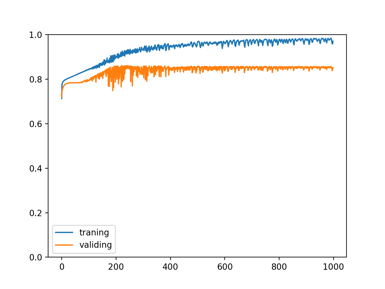
Correct rate after 1000 fixed training:
training accuracy: 0.9706422178819776
validating accuracy: 0.8514168351888657
highest validating accuracy: 0.8607834208011628 from epoch 223
testing accuracy: 0.8603586450219154
And the change trend of accuracy:
Try to add two dropouts to the model, corresponding to the output of the first layer and the second layer (hidden value):
class MyModel(nn.Module):
    """A model for predicting wages according to the code farming conditions"""
    def __init__(self):
        super().__init__()
        self.layer1 = nn.Linear(in_features=8, out_features=200)
        self.layer2 = nn.Linear(in_features=200, out_features=100)
        self.layer3 = nn.Linear(in_features=100, out_features=1)
        self.dropout1 = nn.Dropout(0.2)
        self.dropout2 = nn.Dropout(0.2)

    def forward(self, x):
        hidden1 = self.dropout1(nn.functional.relu(self.layer1(x)))
        hidden2 = self.dropout2(nn.functional.relu(self.layer2(hidden1)))
        y = self.layer3(hidden2)
        return y
Training again at this time will get the following accuracy:
training accuracy: 0.9326518730819225
validating accuracy: 0.8692235469818115
highest validating accuracy: 0.8728838726878166 from epoch 867
testing accuracy: 0.8733032837510109
And the change trend of accuracy:
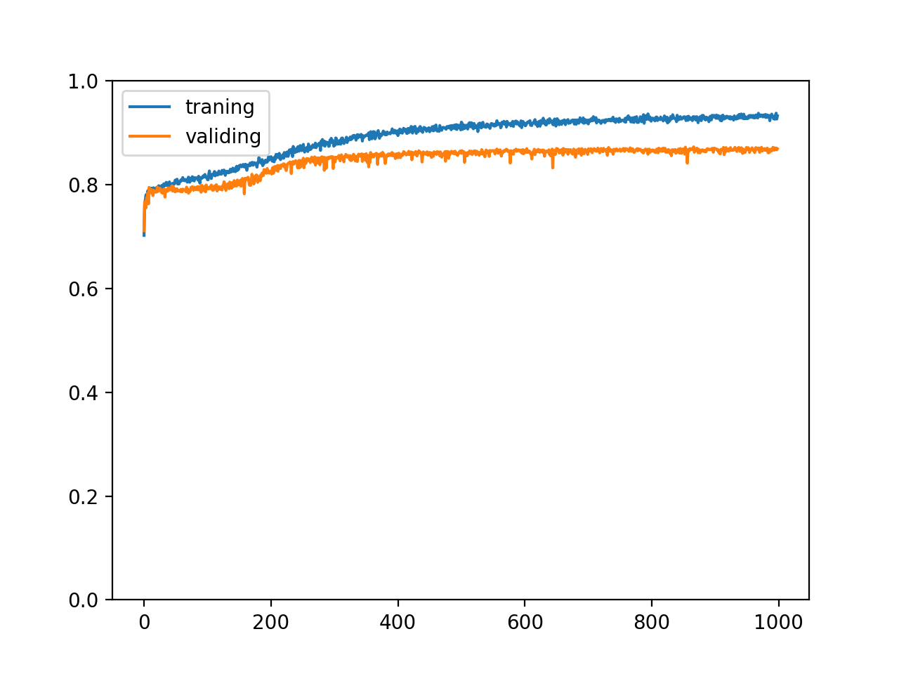
We can see that the accuracy of the training set has not increased blindly, and the accuracy of the verification set and the test set has increased by more than 1% respectively, indicating that Dropout has a certain effect.
When using Dropout, you should pay attention to the following points:
- Dropout should be used for hidden values and cannot be placed in front of the first layer (for input) or behind the last layer (for output)
- Dropout should be placed after the activation function (because the activation function is part of the neuron)
- Dropout should only be used during training. When evaluating or actually using the model, you should call {model Eval() switches the model to evaluation mode to prohibit dropout
- The Dropout function should be defined as a member of the model, which calls {model Eval () can index all Dropout functions corresponding to the model
- There is no optimal value for the shielding ratio of Dropout. You can try several times for the current data and model to find the best result
The original paper proposing the Dropout technique is in here , you can check it if you are interested.
Normalize batches using BatchNorm
BatchNorm is another way to improve the training effect. In some scenarios, it can improve the training efficiency and suppress overfitting. BatchNorm, like Dropout, is used for hidden values and normalizes the values (each column) of each batch. The calculation formula is as follows:
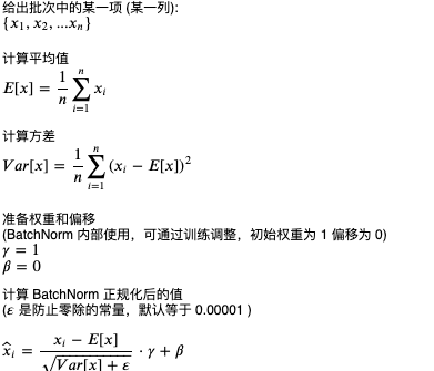
To sum up, let each value in each column subtract the average value of this column, then divide it by the standard deviation of this column, and then adjust it according to a certain proportion.
An example of using BatchNorm in python is as follows:
# Create a batchnorm function, where 3 represents the number of columns
>>> batchnorm = torch.nn.BatchNorm1d(3)

# View the weight and offset inside the batchnorm function
>>> list(batchnorm.parameters())
[Parameter containing:
tensor([1., 1., 1.], requires_grad=True), Parameter containing:
tensor([0., 0., 0.], requires_grad=True)]

# Randomly create a tensor with 10 rows and 3 columns
>>> a = torch.rand((10, 3))
>>> a
tensor([[0.9643, 0.6933, 0.0039],
        [0.3967, 0.8239, 0.3490],
        [0.4011, 0.8903, 0.3053],
        [0.0666, 0.5766, 0.4976],
        [0.4928, 0.1403, 0.8900],
        [0.7317, 0.9461, 0.1816],
        [0.4461, 0.9987, 0.8324],
        [0.3714, 0.6550, 0.9961],
        [0.4852, 0.7415, 0.1779],
        [0.6876, 0.1538, 0.3429]])

# Applying the batchnorm function
>>> batchnorm(a)
tensor([[ 1.9935,  0.1096, -1.4156],
        [-0.4665,  0.5665, -0.3391],
        [-0.4477,  0.7985, -0.4754],
        [-1.8972, -0.2986,  0.1246],
        [-0.0501, -1.8245,  1.3486],
        [ 0.9855,  0.9939, -0.8611],
        [-0.2523,  1.1776,  1.1691],
        [-0.5761, -0.0243,  1.6798],
        [-0.0831,  0.2783, -0.8727],
        [ 0.7941, -1.7770, -0.3581]], grad_fn=<NativeBatchNormBackward>)

# Manually reproduce the calculation of the first column by batchnorm
>>> aa = a[:,:1]
>>> aa
tensor([[0.9643],
        [0.3967],
        [0.4011],
        [0.0666],
        [0.4928],
        [0.7317],
        [0.4461],
        [0.3714],
        [0.4852],
        [0.6876]])
>>> (aa - aa.mean()) / (((aa - aa.mean()) ** 2).mean() + 0.00001).sqrt()
tensor([[ 1.9935],
        [-0.4665],
        [-0.4477],
        [-1.8972],
        [-0.0501],
        [ 0.9855],
        [-0.2523],
        [-0.5761],
        [-0.0831],
        [ 0.7941]])
The code of BatchNorm used to modify the model is as follows:
class MyModel(nn.Module):
    """A model for predicting wages according to the code farming conditions"""
    def __init__(self):
        super().__init__()
        self.layer1 = nn.Linear(in_features=8, out_features=200)
        self.layer2 = nn.Linear(in_features=200, out_features=100)
        self.layer3 = nn.Linear(in_features=100, out_features=1)
        self.batchnorm1 = nn.BatchNorm1d(200)
        self.batchnorm2 = nn.BatchNorm1d(100)
        self.dropout1 = nn.Dropout(0.1)
        self.dropout2 = nn.Dropout(0.1)

    def forward(self, x):
        hidden1 = self.dropout1(self.batchnorm1(nn.functional.relu(self.layer1(x))))
        hidden2 = self.dropout2(self.batchnorm2(nn.functional.relu(self.layer2(hidden1))))
        y = self.layer3(hidden2)
        return y
The learning ratio needs to be adjusted at the same time:
# Create parameter adjuster
optimizer = torch.optim.SGD(model.parameters(), lr=0.05)
The results of 1000 fixed training times are as follows. It can be seen that BatchNorm does not work in this scenario 🤕, Instead, it slows down the learning speed and affects the highest attainable accuracy (you can try increasing the number of training):
training accuracy: 0.9048486271500588
validating accuracy: 0.8341873311996459
highest validating accuracy: 0.8443503141403198 from epoch 946
testing accuracy: 0.8452585405111313
When using BatchNorm, you should pay attention to the following points:
- BatchNorm should be used for hidden values, just like Dropout
- BatchNorm needs to specify the number of hidden values, which should match the output number of the corresponding layer
- BatchNorm should be placed in front of Dropout. Some people choose to put BatchNorm before the activation function, while others choose to put it after the activation function
- Linear => ReLU => BatchNorm => Dropout
- Linear => BatchNorm => ReLU => Dropout
- BatchNorm should only be used during training, just like Dropout
- The BatchNorm function should be defined as a member of the model, just like Dropout
- When using BatchNorm, the shielding ratio of Dropout should be reduced accordingly
- Some scenes may not be applicable to BatchNorm (it is said that it is more applicable to object recognition and picture classification), which requires practice to get true knowledge ☭
The original paper that proposed BatchNorm technique here , you can check it if you are interested.
Understand the eval and train patterns of the model
In the previous example, we used the "eval" and "train" functions to switch the model to the evaluation mode and training mode. The evaluation mode will disable automatic differentiation, Dropout and BatchNorm. How are these two modes implemented?
pytorch's models are based on {torch nn. Module is not only a model defined by ourselves, NN Sequential, nn.Linear, nn.ReLU, nn.Dropout, nn. The types of batchnorm1d and so on are based on batch torch nn. Module,torch.nn.Module , has a , training , member to represent whether the model is in training mode. The , eval , function is used to recursively set , training , of all , modules , to False, and the train , function is used to recursively set , training , of all. We can manually set this member to see if it can have the same effect:
>>> a = torch.tensor(range(1, 11), dtype=torch.float)
>>> dropout = torch.nn.Dropout(0.2)

>>> dropout.training = False
>>> dropout(a)
tensor([ 1.,  2.,  3.,  4.,  5.,  6.,  7.,  8.,  9., 10.])

>>> dropout.training = True
>>> dropout(a)
tensor([ 1.2500,  2.5000,  3.7500,  0.0000,  0.0000,  7.5000,  8.7500, 10.0000,
         0.0000, 12.5000])
After understanding this, you can add code to the model that only executes during training or evaluation, according to {self Training {judgment is enough.
Final code
The final code for predicting wages according to the code farming conditions is as follows:
import os
import sys
import pandas
import torch
import gzip
import itertools
from torch import nn
from matplotlib import pyplot

class MyModel(nn.Module):
    """A model for predicting wages according to the code farming conditions"""
    def __init__(self):
        super().__init__()
        self.layer1 = nn.Linear(in_features=8, out_features=200)
        self.layer2 = nn.Linear(in_features=200, out_features=100)
        self.layer3 = nn.Linear(in_features=100, out_features=1)
        self.batchnorm1 = nn.BatchNorm1d(200)
        self.batchnorm2 = nn.BatchNorm1d(100)
        self.dropout1 = nn.Dropout(0.1)
        self.dropout2 = nn.Dropout(0.1)

    def forward(self, x):
        hidden1 = self.dropout1(self.batchnorm1(nn.functional.relu(self.layer1(x))))
        hidden2 = self.dropout2(self.batchnorm2(nn.functional.relu(self.layer2(hidden1))))
        y = self.layer3(hidden2)
        return y

def save_tensor(tensor, path):
    """preservation tensor Object to file"""
    torch.save(tensor, gzip.GzipFile(path, "wb"))

def load_tensor(path):
    """Read from file tensor object"""
    return torch.load(gzip.GzipFile(path, "rb"))

def prepare():
    """Preparation training"""
    # After the dataset is converted to tensor, it will be saved in the data folder
    if not os.path.isdir("data"):
        os.makedirs("data")

    # Read the original data set from csv, and read 2000 rows each time in batches
    for batch, df in enumerate(pandas.read_csv('salary.csv', chunksize=2000)):
        dataset_tensor = torch.tensor(df.values, dtype=torch.float)

        # Normalized input and output
        dataset_tensor *= torch.tensor([0.01, 1, 0.01, 0.2, 0.2, 0.2, 0.2, 0.2, 0.0001])

        # Segmentation training set (60%), verification set (20%) and test set (20%)
        random_indices = torch.randperm(dataset_tensor.shape[0])
        traning_indices = random_indices[:int(len(random_indices)*0.6)]
        validating_indices = random_indices[int(len(random_indices)*0.6):int(len(random_indices)*0.8):]
        testing_indices = random_indices[int(len(random_indices)*0.8):]
        training_set = dataset_tensor[traning_indices]
        validating_set = dataset_tensor[validating_indices]
        testing_set = dataset_tensor[testing_indices]

        # Save to hard disk
        save_tensor(training_set, f"data/training_set.{batch}.pt")
        save_tensor(validating_set, f"data/validating_set.{batch}.pt")
        save_tensor(testing_set, f"data/testing_set.{batch}.pt")
        print(f"batch {batch} saved")

def train():
    """Start training"""
    # Create model instance
    model = MyModel()

    # Create loss calculator
    loss_function = torch.nn.MSELoss()

    # Create parameter adjuster
    optimizer = torch.optim.SGD(model.parameters(), lr=0.05)

    # Record the change of accuracy of training set and verification set
    traning_accuracy_history = []
    validating_accuracy_history = []

    # Record the highest validation set accuracy
    validating_accuracy_highest = 0
    validating_accuracy_highest_epoch = 0

    # Tool functions for reading batches
    def read_batches(base_path):
        for batch in itertools.count():
            path = f"{base_path}.{batch}.pt"
            if not os.path.isfile(path):
                break
            yield load_tensor(path)

    # Tool function for calculating accuracy
    def calc_accuracy(actual, predicted):
        return max(0, 1 - ((actual - predicted).abs() / actual.abs()).mean().item())

    # Start the training process
    for epoch in range(1, 10000):
        print(f"epoch: {epoch}")

        # Train and modify the parameters according to the training set
        # Switching the model to training mode will enable automatic differentiation, batchnorm and Dropout
        model.train()
        traning_accuracy_list = []
        for batch in read_batches("data/training_set"):
            # Splitting small batches is helpful to generalize the model
             for index in range(0, batch.shape[0], 100):
                # Divide input and output
                batch_x = batch[index:index+100,:-1]
                batch_y = batch[index:index+100,-1:]
                # Calculate predicted value
                predicted = model(batch_x)
                # Calculate loss
                loss = loss_function(predicted, batch_y)
                # Deriving function value from loss automatic differentiation
                loss.backward()
                # Use the parameter adjuster to adjust the parameters
                optimizer.step()
                # Clear leading function value
                optimizer.zero_grad()
                # Record the accuracy of this batch, torch no_ Grad stands for temporarily disabling the automatic differentiation function
                with torch.no_grad():
                    traning_accuracy_list.append(calc_accuracy(batch_y, predicted))
        traning_accuracy = sum(traning_accuracy_list) / len(traning_accuracy_list)
        traning_accuracy_history.append(traning_accuracy)
        print(f"training accuracy: {traning_accuracy}")

        # Check validation set
        # Switching the model to validation mode will disable automatic differentiation, batchnorm and Dropout
        model.eval()
        validating_accuracy_list = []
        for batch in read_batches("data/validating_set"):
            validating_accuracy_list.append(calc_accuracy(batch[:,-1:],  model(batch[:,:-1])))
        validating_accuracy = sum(validating_accuracy_list) / len(validating_accuracy_list)
        validating_accuracy_history.append(validating_accuracy)
        print(f"validating accuracy: {validating_accuracy}")

        # Record the highest accuracy of the verification set and the current model state, and judge whether the record is still not refreshed after 100 training
        if validating_accuracy > validating_accuracy_highest:
            validating_accuracy_highest = validating_accuracy
            validating_accuracy_highest_epoch = epoch
            save_tensor(model.state_dict(), "model.pt")
            print("highest validating accuracy updated")
        elif epoch - validating_accuracy_highest_epoch > 100:
            # After 100 times of training, you still didn't refresh the record and ended the training
            print("stop training because highest validating accuracy not updated in 100 epoches")
            break

    # Use the model state at the highest accuracy
    print(f"highest validating accuracy: {validating_accuracy_highest}",
        f"from epoch {validating_accuracy_highest_epoch}")
    model.load_state_dict(load_tensor("model.pt"))

    # Check test set
    testing_accuracy_list = []
    for batch in read_batches("data/testing_set"):
        testing_accuracy_list.append(calc_accuracy(batch[:,-1:],  model(batch[:,:-1])))
    testing_accuracy = sum(testing_accuracy_list) / len(testing_accuracy_list)
    print(f"testing accuracy: {testing_accuracy}")

    # Display the correct rate change of training set and verification set
    pyplot.plot(traning_accuracy_history, label="traning")
    pyplot.plot(validating_accuracy_history, label="validing")
    pyplot.ylim(0, 1)
    pyplot.legend()
    pyplot.show()

def eval_model():
    """Use the trained model"""
    parameters = [
        "Age",
        "Gender (0: Male, 1: Female)",
        "Years of work experience",
        "Java Skill (0 ~ 5)",
        "NET Skill (0 ~ 5)",
        "JS Skill (0 ~ 5)",
        "CSS Skill (0 ~ 5)",
        "HTML Skill (0 ~ 5)"
    ]

    # Create a model instance, load the trained state, and then switch to verification mode
    model = MyModel()
    model.load_state_dict(load_tensor("model.pt"))
    model.eval()

    # Query input and predict output
    while True:
        try:
            x = torch.tensor([int(input(f"Your {p}: ")) for p in parameters], dtype=torch.float)
            # Normalized input
            x *= torch.tensor([0.01, 1, 0.01, 0.2, 0.2, 0.2, 0.2, 0.2])
            # Conversion to a matrix with one row and one column is not required here, but it is recommended because not all models support non batch input
            x = x.view(1, len(x))
            # Prediction output
            y = model(x)
            # Arc normalized output
            y *= 10000
            print("Your estimated salary:", y[0,0].item(), "\n")
        except Exception as e:
            print("error:", e)

def main():
    """Main function"""
    if len(sys.argv) < 2:
        print(f"Please run: {sys.argv[0]} prepare|train|eval")
        exit()

    # Assign an initial value to the random number generator so that each run can generate the same random number
    # This is to make the process reproducible, or you can choose not to do so
    torch.random.manual_seed(0)

    # Select the operation according to the command line parameters
    operation = sys.argv[1]
    if operation == "prepare":
        prepare()
    elif operation == "train":
        train()
    elif operation == "eval":
        eval_model()
    else:
        raise ValueError(f"Unsupported operation: {operation}")

if __name__ == "__main__":
    main()
The final training results are as follows: the accuracy of verification set and test set reaches 94.3% (93.3% and 93.1% respectively in the previous article):
epoch: 848
training accuracy: 0.929181088420252
validating accuracy: 0.9417830203473568
stop training because highest validating accuracy not updated in 100 epoches
highest validating accuracy: 0.9437697219848633 from epoch 747
testing accuracy: 0.9438129015266895
The accuracy changes are as follows:
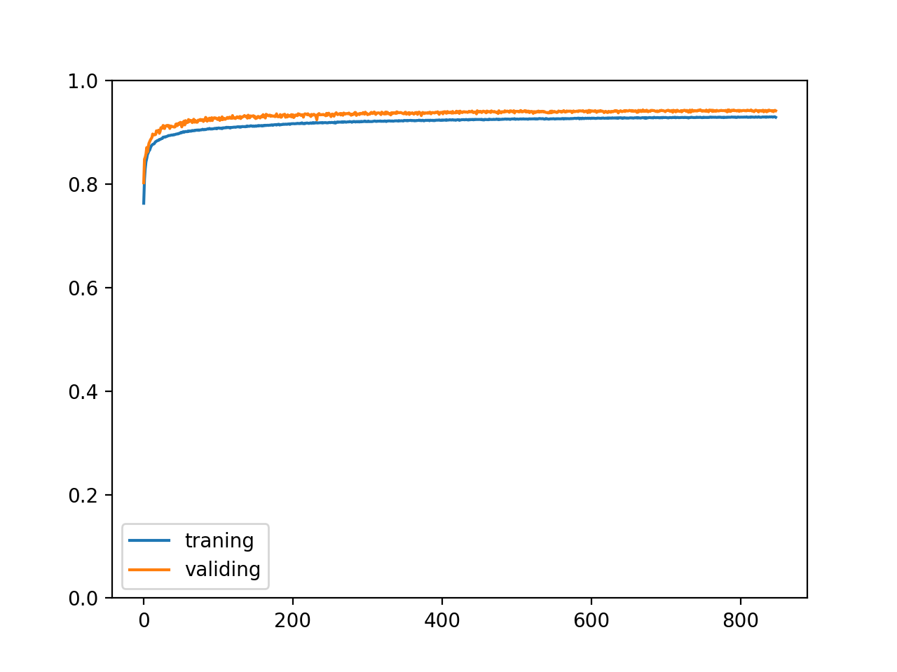
It's a complete success 🥳.
Write at the end
In this article, we see various ways to improve the training process and training effect, and predict the wages of various yard farmers 🙀, Then we can try to do something different. The next chapter will introduce the recursive models RNN, LSTM and GRU, which can be used to process data of variable length, and realize the functions of classification according to context, prediction of trend, automatic completion and so on.