In today's article, we are formally exposed to the theoretical basis of deep learning - machine learning

1, Machine learning classification

1. Based on subject classification
Statistics, artificial intelligence, information theory, control theory
2. Classification based on learning patterns
Inductive learning, explanatory learning and feedback learning
3. Classification based on application domain
Expert system, data mining, image recognition, artificial intelligence, natural language processing

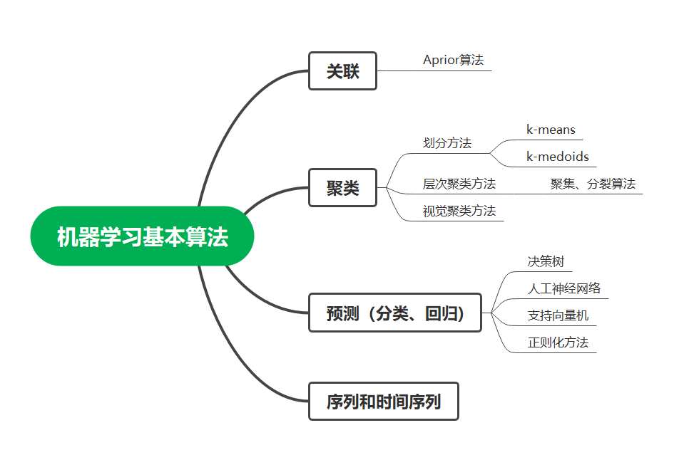
2, Basic algorithm of machine learning

A complete machine learning project includes the following contents:
1. Input data: naturally collected data sets
2. Feature extraction: extract the feature values of data in a variety of ways
3. Model design: the most important part of machine learning
4. Data prediction: realize the prediction through the use and understanding of the trained mode.

Basic algorithm classification:
1. Unsupervised learning: the method of complete black box training has no difference and identification for the input data
2. Supervised learning: data is artificially classified, marked and distinguished
3. Semi supervised learning: training with mixed labeled and unlabeled data
4. Reinforcement learning: input different identification data

3, Theoretical basis of algorithm

For machine learning, the most important part is data collection and algorithm design.

When we were in primary school, we knew that calculating the area of a circle can be approximated by inscribed polygons. Our machine learning is similar to this. In fact, this is also the mathematical basis of our so-called calculus.

1. Basic theory of machine learning -- function approximation

For machine learning, the theoretical basis of machine learning algorithm is function approximation. The specific basic algorithm will be discussed in the subsequent reading notes.

Today, we mainly introduce the function approximation in machine learning, among which the most commonly used is regression algorithm.

2. Regression algorithm

First of all, we should have an understanding of regression: regression analysis is a statistical analysis method to determine the interdependent quantitative relationship between two or more variables.
According to the relationship between independent variables and dependent variables, it can be divided into linear regression analysis and nonlinear regression analysis.

In short, regression algorithm is also a prediction algorithm based on existing data (learning content of primary mathematics in senior high school). The purpose is to study the causal relationship between data characteristic factors and results.

The sister of linear regression ---- logical regression

Logistic regression is mainly used in the field of classification. Its main function is to classify and identify data of different properties.
Let's take a look at the implementation code (those who need data sets can be private): (reprinted here from Logistic)

import matplotlib
import matplotlib.pyplot as plt
import csv
import numpy as np
import math

def loadDataset():
    data=[]
    labels=[]
    with open('C:\\Users\\AWAITXM\\Desktop\\logisticDataset.txt','r') as f:  # "C:\Users\AWAITXM\Desktop\logisticDataset.txt"
        reader = csv.reader(f,delimiter='\t')
        for row in reader:
            data.append([1.0, float(row[0]), float(row[1])])
            labels.append(int(row[2]))
    return data,labels

def plotBestFit(W):
    # Draw the training set data in the form of coordinates
    dataMat,labelMat=loadDataset()
    dataArr = np.array(dataMat)
    n = np.shape(dataArr)[0]
    xcord1 = []
    ycord1 = []
    xcord2 = []
    ycord2 = []
    for i in range(n):
        if int(labelMat[i])== 1:
            xcord1.append(dataArr[i,1]); ycord1.append(dataArr[i,2])
        else:
            xcord2.append(dataArr[i,1]); ycord2.append(dataArr[i,2])
    fig = plt.figure()
    ax = fig.add_subplot(111)
    ax.scatter(xcord1, ycord1, s=30, c='red', marker='s')
    ax.scatter(xcord2, ycord2, s=30, c='green')

    # Draw the classification boundary
    x = np.arange(-3.0,3.0,0.1)
    y = (-W[0]-W[1]*x)/W[2]
    ax.plot(x,y)
    plt.show()

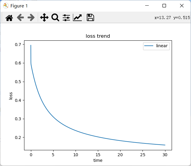
def plotloss(loss_list):
    x = np.arange(0,30,0.01)
    plt.plot(x,np.array(loss_list),label = 'linear')

    plt.xlabel('time')       # Number of gradient descent
    plt.ylabel('loss')       # magnitude of the loss
    plt.title('loss trend')         # The loss value is constantly updated and changing with W
    plt.legend()               # Graphic legend
    plt.show()

def main():
    # Read the data in the training set (txt file),
    data, labels = loadDataset()
    # Convert the data into the form of matrix for later calculation
    # Constructing characteristic matrix X
    X = np.array(data)
    # Build label matrix y
    y = np.array(labels).reshape(-1,1)
    # Randomly generate a w parameter (weight) matrix The function of reshape((-1,1)) is not to know how many rows there are, but to become a column
    W = 0.001*np.random.randn(3,1).reshape((-1,1))
    # m indicates how many groups of training data there are in total
    m = len(X)
    # The learning rate of gradient descent is defined as 0.03
    learn_rate = 0.03

    loss_list = []
    # Realize the gradient descent algorithm, constantly update W, obtain the optimal solution, and minimize the loss value of the loss function
    for i in range(3000):
        # The most important thing is to use numpy matrix calculation to complete the calculation of hypothesis function, loss function and gradient descent
        # Calculate the hypothetical function h(w)x
        g_x = np.dot(X,W)
        h_x = 1/(1+np.exp(-g_x))

        # Calculate the loss value loss of Cost Function
        loss = np.log(h_x)*y+(1-y)*np.log(1-h_x)
        loss = -np.sum(loss)/m
        loss_list.append(loss)

        # Update W weight with gradient descent function
        dW = X.T.dot(h_x-y)/m
        W += -learn_rate*dW

    # Get updated W, visualization
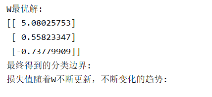
    print('W Optimal solution:')
    print(W)
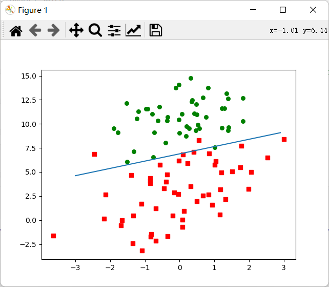
    print('The final classification boundary:')
    plotBestFit(W)
    print('Loss value with W Constantly updated and changing trend:')
    plotloss(loss_list)

    # Define a test data and calculate which category it belongs to
    test_x = np.array([1,-1.395634,4.662541])
    test_y = 1/(1+np.exp(-np.dot(test_x,W)))
    print(test_y)

#     print(data_arr)
if __name__=='__main__':
    main()

The operation results are shown in the figure below:



I also refer to this specific tutorial. You can also have a look: logistic regression

As for the loss function and cost function, you can refer to this blog: Cost function

3. Other algorithms - decision tree

The decision tree is relatively easy to understand, that is, the process of reasoning from the root of the tree structure layer by layer.

Application of decision tree theory (from network):
As a girl, your mother has been very worried about your life. Today she will introduce you to someone else. You casually asked: how old?
She said: 26
You ask: are you handsome?
She said: very handsome.
You ask: is the income high?
She said: not very high, medium.
You ask: how about your education?
She said: what about graduate students from famous universities?
You say: OK, I'll see you.

What is a decision tree? In fact, the basic logic of the decision tree is involved in the problem just now.
When you ask, "how old?" In fact, the first decision node of the "blind date decision tree" is started. This decision node has two branches:
First, over 30? Oh, too old, then it's gone;
Second, under 30? Oh, age is OK. Then you'll ask, "are you handsome?"
This is another decision-making node, "to the ugly level", then don't see it. If it is at least medium, then go down to the third decision node "is the income high?" No money? That's unbearable. Then there is the fourth decision node "is it a high degree?". Yes? Great. The young man has a bright future. See you then.

Through the four decision-making nodes "age, appearance, income and progress", you exclude the "old, ugly and poor people who are not progressive", and select the "handsome guy under the age of 30, with medium income, but very progressive, who is studying at Munger College".
This set of decision-making tools, which branch layer by layer and advance continuously like a tree, is the "decision tree".

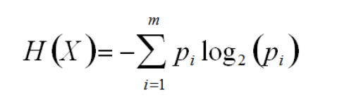
The algorithmic basis of decision tree -- information entropy

Information entropy is a measure of uncertain information in events. In an event or attribute, the greater the information entropy, the greater the uncertain information contained, and the more beneficial it is to the calculation of data analysis. Therefore, the information entropy always selects the attribute with the highest information entropy in the current event as the attribute to be tested.

So, how to calculate information entropy? This is a probability calculation problem:

Presentation data:

Gender (x)	Test result (y)
male	excellent
female	excellent
male	difference
female	excellent
male	excellent

The information entropy of X is calculated as:
P (male) = 3 / 5 = 0.6
P (female) = 2 / 5 = 0.4
According to the above calculation formula:
The information entropy of column x is: H (x) = - (0.6 * log2(0.6) + 0.4 * log2(0.4)) = 0.97
The information entropy of Y is calculated as:
P (excellent) = 4 / 5 = 0.8
P (difference) = 1 / 5 = 0.2
The information entropy of column x is: H (x) = - (0.8 * log2(0.8) + 0.2 * log2(0.2)) = 0.72
(data from link) Calculation of information entropy)

That's all for today's record. See you next time!