preface

K-nearest neighbor (k-NN) is a basic classification and regression method. It is one of the simplest algorithms in data mining technology. Its core function is to solve the supervised classification problem.

KNN can quickly and efficiently solve the prediction classification problem based on special data sets, but it does not produce models.

The input of k-nearest neighbor method is the feature vector of the instance, which corresponds to the points in the feature space; The output is the category of the instance, and multiple classes can be selected.

There are three basic elements of k-nearest neighbor method: k-value selection, distance measurement and classification decision rules.

Algorithm process

1 calculate the distance between each sample point in the training sample and the test sample;
2 sort all the distance values above;
3. Select the first k samples with the minimum distance;
4 vote according to the labels of these k samples to get the final classification category.

Distance measurement

The distance between two instance points in feature space is the reflection of the similarity of two instance points.

In distance models, such as KNN, there are many common distance measurement methods. Such as Euclidean distance, Manhattan distance, minkovsky distance, Chebyshev distance and cosine distance. Euclidean distance is the most common.

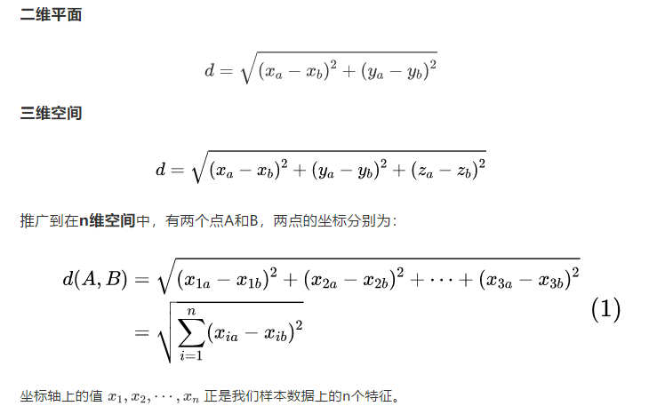
• Euclidean distance

In Euclidean space, the distance between two or more points is also called Euclidean metric.

• Manhattan distance

Manhattan distance, formally referred to as urban block distance, also known as street distance, is the sum of the distance of the projection generated by the line segment formed by the fixed rectangular coordinates in Euclidean space. Its calculation method is equivalent to the first power expression of Euclidean distance, and its basic calculation formula is as follows:

• Minkowski distance

Min's distance is not a kind of distance, but the definition of a group of distances. It is a general expression of multiple distance measurement formulas. Both European distance and Manhattan distance can be regarded as a special case of Minkowski distance.

Where p is a variable parameter:

• When p=1, it is Manhattan distance;
• When p=2, it is Euclidean distance;
• When p →∞, it is the Chebyshev distance.

Therefore, according to different variable parameters, min distance can represent the distance of a certain class / species.

Min's distance, including Manhattan distance, Euclidean distance and Chebyshev distance, has obvious disadvantages.
e.g. two dimensional samples (height [unit: cm], weight [unit: kg]). There are three samples: a(180,50), b(190,50), c(180,60). Then the Min distance between a and b (whether Manhattan distance, Euclidean distance or Chebyshev distance) is equal to the Min distance between a and c. But in fact, 10cm of height is not equal to 10kg of weight.
Disadvantages of Min's distance:
(1) Treat the scale of each component, that is, the "unit" in the same way;
(2) The distribution of each component (expectation, variance, etc.) may be different without considering.

• Chebyshev distance

In chess, the king can go straight, horizontal and oblique, so the king can move to any of the eight adjacent squares in one step. How many steps does it take for the king to walk from the grid (xa,ya) to the grid (xb,yb)? This distance is called Chebyshev distance.

• Cosine distance

Cosine similarity measures the difference between two samples by the cosine value of the angle between two vectors in vector space. The closer the cosine value is to 1, the closer the angle between the two vectors is to 0 degrees, and the more similar the two vectors are. In geometry, the cosine of the included angle can be used to measure the difference between the directions of two vectors; In machine learning, this concept is used to measure the difference between sample vectors.

K value selection

The choice of k value will have a significant impact on the results of KNN algorithm.

• The decrease of k value means that the overall model becomes complex, and the learner is vulnerable to over fitting due to the noise in the training data.
• The increase of K value means that the overall model becomes simple. If K is too large, the nearest neighbor classifier may classify the test samples incorrectly, because the k nearest neighbors may contain data points that are far away and not of the same kind.

In the application, the k value is generally a smaller value, and the cross validation is usually used to select the optimal k value.

Classification decision rules

According to the principle of "the minority obeys the majority, one count counts one vote", the label category with the largest number is the label category of x. The principle involved is "the closer the more similar", which is also the basic assumption of KNN.

Insufficient algorithm

As a simple algorithm, KNN algorithm has some shortcomings.

• There is no obvious training process. It is a typical representative of "lazy learning". All it does in the training stage is to save the samples. If the training set is large, a large amount of storage space must be used, and the training time overhead is zero.
• KNN must calculate the distance to each training data point for each test point, and these distance points involve all features. When the dimension of data is large and the amount of data is also large, KNN calculation will become a curse.

kd-tree

Due to the above shortcomings, in order to improve the speed of KNN search, special data storage forms can be used to reduce the number of distance calculations. kd tree is a method of storing data in the form of binary tree.

kd tree is a partition of k-dimensional space. Constructing kd tree is equivalent to continuously dividing k-dimensional space with a hyperplane perpendicular to the coordinate axis to form a series of k-dimensional hypermatrix regions. Each node of kd tree corresponds to a hypermatrix region.

code implementation

# From sklearn Class of KNN classifier imported from neighbors
from sklearn.neighbors import KNeighborsClassifier
# Instantiate a knn classifier object through a class
# Class
# KNeighborsClassifier(n_neighbors=5,weights='uniform',algorithm='auto',leaf_size=30,p=2, metric='minkowski',metric_params=None,n_jobs=None,**kwargs,)
knn_clf = KNeighborsClassifier(n_neighbors=k)
# Through the object tuning fit() method, the training set and training model are introduced
knn_clf.fit(X_train, y_train)X
# The trained model can be imported into the test set through other interfaces to view the model effect
knn_clf.score(X_test, y_test)
# Prediction results
knn_clf.predict(X_test)
knn_clf.predict_proba(X_test)

Realize unsupervised nearest neighbor KNN learning. It acts as a unified interface for three different nearest neighbors algorithms: BallTree, KDTree and sklear metrics. Pairwise routine violence algorithm.

The selection of neighbor search algorithm is controlled by the keyword 'algorithm', which must be one of ['auto', 'ball_tree', 'kd_tree', 'brute]. When the default value is' auto ', the algorithm tries to determine the best method from the training data.

Case practice

1. Iris

Data: Iris dataset
https://scikit-learn.org/stable/modules/generated/sklearn.datasets.load_iris.html

import numpy as np
import pandas as pd
import matplotlib.pyplot as plt
import matplotlib as mpl
from sklearn.model_selection import train_test_split
from sklearn.metrics import accuracy_score
from matplotlib.colors import ListedColormap
#Import iris data
from sklearn.datasets import load_iris
iris = load_iris()
X=iris.data[:,:2] #Only the first two columns are taken
y=iris.target

X_train, X_test, y_train, y_test = train_test_split(X, y, stratify=y,random_state=42) #Partition data, random_state fixed partition method
#Import model
from sklearn.neighbors import KNeighborsClassifier 
#Training model
n_neighbors = 5
knn = KNeighborsClassifier(n_neighbors=n_neighbors)
knn.fit(X_train, y_train)
y_pred = knn.predict(X_test)
#View each score
print("y_pred",y_pred)
print("y_test",y_test)
print("score on train set", knn.score(X_train, y_train))
print("score on test set", knn.score(X_test, y_test))
print("accuracy score", accuracy_score(y_test, y_pred))

# visualization

# Custom colormap
def colormap():
    return mpl.colors.LinearSegmentedColormap.from_list('cmap', ['#FFC0CB','#00BFFF', '#1E90FF'], 256)

x_min, x_max = X[:, 0].min() - 1, X[:, 0].max() + 1
y_min, y_max = X[:, 1].min() - 1, X[:, 1].max() + 1
axes=[x_min, x_max, y_min, y_max]
xp=np.linspace(axes[0], axes[1], 500) #Abscissa of uniform 500
yp=np.linspace(axes[2], axes[3],500) #Uniform 500 ordinates
xx, yy=np.meshgrid(xp, yp) #Generate 500X500 grid points
xy=np.c_[xx.ravel(), yy.ravel()] #Splice according to lines and standardize the format of coordinate points
y_pred = knn.predict(xy).reshape(xx.shape) #Tile after training

# Visualization method I
plt.figure(figsize=(15,5),dpi=100)
plt.subplot(1,2,1)
plt.contourf(xx, yy, y_pred, alpha=0.3, cmap=colormap())
#Draw three types of points
p1=plt.scatter(X[y==0,0], X[y==0, 1], color='blue',marker='^')
p2=plt.scatter(X[y==1,0], X[y==1, 1], color='green', marker='o')
p3=plt.scatter(X[y==2,0], X[y==2, 1], color='red',marker='*')
#Set comments
plt.legend([p1, p2, p3], iris['target_names'], loc='upper right',fontsize='large')
#Set title
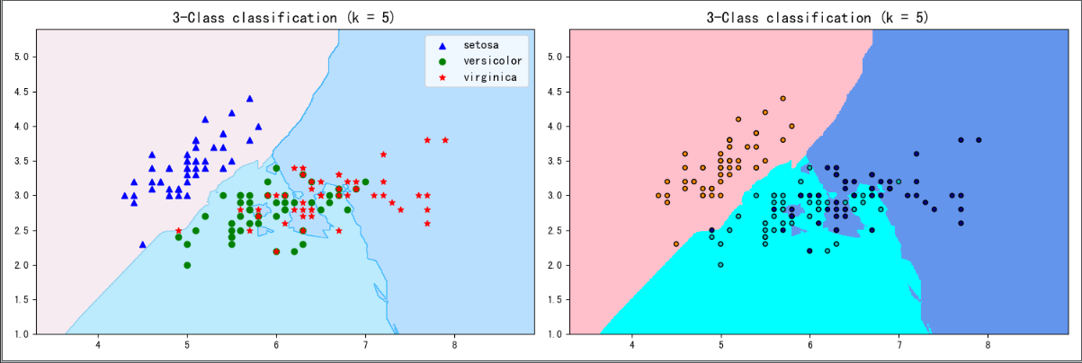
plt.title(f"3-Class classification (k = {n_neighbors})", fontdict={'fontsize':15} )

# Visualization method II
plt.subplot(1,2,2)
cmap_light = ListedColormap(['pink', 'cyan', 'cornflowerblue'])
cmap_bold = ListedColormap(['darkorange', 'c', 'darkblue'])
plt.pcolormesh(xx, yy, y_pred, cmap=cmap_light)

# Plot also the training points
plt.scatter(X[:, 0], X[:, 1], c=y, cmap=cmap_bold,
                edgecolor='k', s=20)
plt.xlim(xx.min(), xx.max())
plt.ylim(yy.min(), yy.max())
plt.title(f"3-Class classification (k = {n_neighbors})" ,fontdict={'fontsize':15})
plt.show()

Output result:

2. Breast cancer

Data: breast cancer dataset
https://scikit-learn.org/stable/modules/generated/sklearn.datasets.load_breast_cancer.html

• get data

# Import class and other packages of breast cancer dataset
from sklearn.datasets import load_breast_cancer
from sklearn.neighbors import KNeighborsClassifier
from sklearn.model_selection import train_test_split
# Instantiating a breast cancer dataset object
breast_cancer= load_breast_cancer()
# View data
breast_cancer
# Data characteristics, return a two-dimensional array
X = breast_cancer['data']
X = pd.DataFrame(X)
name = ['Average radius','Average texture','Average perimeter','Average area','Average smoothness','Average compactness','Average concavity','Average concave point','Average symmetry','Average fractal dimension','Radius error','Texture error','Perimeter error','Area error','Smoothness error','Compactness error','Concavity error','Concave error','Symmetry error','Fractal dimension error','Worst radius','Worst texture','Worst boundary','Worst area','Worst smoothness','Worst compactness','Worst depression','Worst concave point','Worst symmetry','Worst fractal dimension']
X.columns = name

# The label of the data and returns a one-dimensional array
y = breast_cancer['target']
# Partition data, random_state fixed partition method
X_train, X_test, y_train, y_test = train_test_split(X, y, stratify=y,random_state=42) 

• Establish, train and test models

# Instantiate a knn classifier with five nearest neighbors
knn_clf = KNeighborsClassifier(n_neighbors=5)
# Training model
knn_clf.fit(X_train, y_train)
# Accuracy of test model
knn_clf.score(X_test, y_test)
# 0.9590643274853801

The nearest neighbor k here is 5, and the result is 0.9590643274853801.

Now we need to think about two questions:

1. As mentioned earlier, the size of k value will affect the effect of the model. How to choose the appropriate k value?

2. Whether the model score can be further improved, and what factors affect it?

• Data preprocessing

The data we use is sklearn Datasets data sets are 'perfect' data and do not require routine data preprocessing (including missing values, outliers, duplicate values, etc.).

However, KNN is a distance model, and the inconsistent dimension of data will seriously affect its effect. In the model, there is a characteristic sum of squares in the calculation formula of Euclidean distance:

If the value of a feature is so large that it masks the influence of the distance between features on the total distance, the distance model can not distinguish different types of features well.

Therefore, when using KNN classifier, the data set needs to be de dimensioned first. That is to compress all data into the same range.

The main purpose of data normalization or standardization is to eliminate the influence of dimension on distance model, accelerate the iterative speed of gradient descent algorithm and make it find the optimal solution faster.

# Import normalization class
from sklearn.preprocessing import MinMaxScaler
mms = MinMaxScaler() # Instantiate object
mms.fit(X_train) # This step is to learn the training set and generate the minimum and range on the training set
X_train = mms.transform(X_train) # Normalize the training set with the minimum and range on the training set
X_test = mms.transform(X_test) # Normalize the test set with the minimum and range on the training set

Before normalization:

After normalization:

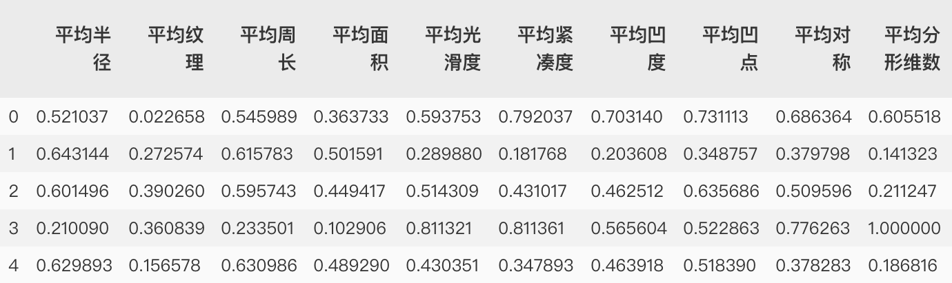
After normalization and other data are brought into the model, the score after training is 0.986013986013986, which is much higher than that of the model before normalization.

• Model tuning

K-fold cross validation

It is the longest cross validation method, which divides the data into N copies, and successively uses one of them as the test set and the other n-1 copies as the training set. In this way, n accuracy rates will appear, and we will average these n accuracy rates. If the average accuracy is high, it means that the generalization ability is stronger.

K-fold cross validation divides the data in order. Therefore, before using cross validation, you need to check whether the labels of the data are in order. If there is order, you need to disrupt the original order, or change the cross validation method. For example, ShuffleSplit doesn't care whether the data itself is in order.

All cross validation is based on the division of training set and test set, but focuses on different directions:

1. KFold is to take the training set and test set in order.
2. ShuffleSplit focuses on Distributing the test set in all directions of the data.
3. Structured kfold believes that training data and test data must account for the same proportion in each label classification.

from sklearn.model_selection import cross_val_score as cvs
L = []
for k in range(1, 21):
 knn_clf = KNeighborsClassifier(n_neighbors=k)
 result = cvs(knn_clf,X_train, # Using training sets
               y_train,
              cv = 5) # 5-fold cross validation
    result_mean = result.mean()
    result_var = result.var()
    L.append((k, result_mean, result_var))
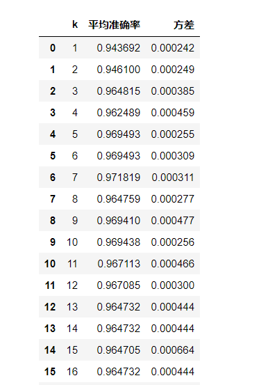
score = pd.DataFrame(L)
score.columns = ['k', 'Average accuracy', 'variance']
score

Output result:

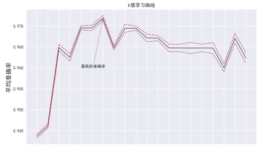
• Draw learning curve

The parameter learning curve is a curve with different parameter values as abscissa and the model results under different parameter values as ordinate. The parameter value of the best performance point of the model is selected as the value of this parameter.

import matplotlib.pyplot as plt
plt.style.use('seaborn')
plt.rcParams['font.sans-serif']=['Simhei'] #Display Chinese 
plt.rcParams['axes.unicode_minus']=False  #Show negative sign
plt.figure(figsize=(8, 6), dpi=100)
plt.plot(score.k, score.Average accuracy)
# Draw two more curves that deviate from the mean by twice the variance
plt.plot(score.k, score.Average accuracy+2*score.variance, linestyle='**', color='r')
plt.plot(score.k, score.Average accuracy-2*score.variance, linestyle='--', color='r')
plt.xticks(score.k)
plt.xlabel('k value', fontsize=20)
plt.ylabel('Average accuracy', fontsize=20)
plt.title("k Value learning curve")
# plt.savefig('learning_curve_picture.jpeg')

Output result:

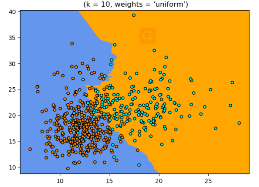
• Important parameters
  weights {'uniform', 'distance'} or callable, default='uniform'

Another basic assumption of KNN classification model: even for the nearest K points, the distance between each point and the classification target point is still far and near, and the near points are often more likely to belong to the same category as the target classification points.

The basic nearest neighbor classification uses a unified weight: the value assigned to the query point is calculated from the simple majority vote of the nearest neighbor. In some environments, it is best to weight the neighbors, so that the closer the neighbors, the more conducive to fitting.

The parameter used to decide whether to use distance as the penalty factor. The default is "uniform".
"uniform": one point one vote
"Distance": the weight of the distance between each point and the test point is calculated based on the reciprocal of the distance between each point and the test point, so that the sample points closer to the test point have greater influence than those farther away from the test point

There are many methods to select the penalty factor. The most commonly used is to weight the action of each nearest neighbor according to its different distance. The weighting method is the set weight, and the weight calculation formula is the reciprocal of the distance.

tips: the optimization method of the model is only in theory. Optimization will improve the discrimination effectiveness of the model, but whether it can play a role in the process of practical application essentially depends on the consistency between the optimization method and the actual data. If there are a large number of outliers in the data itself, using distance as the punishment factor will have a better effect, otherwise.

import numpy as np
import matplotlib.pyplot as plt
from matplotlib.colors import ListedColormap
from sklearn import neighbors, datasets

n_neighbors = 10
h = .02  
breast_cancer= datasets.load_breast_cancer()
X = breast_cancer['data'][:, :2]
y = breast_cancer['target']

cmap_light = ListedColormap(['orange', 'cornflowerblue'])
cmap_bold = ListedColormap([ 'darkblue', 'darkorange'])

p1=plt.figure(figsize=(15,5),dpi=100) 
num = 1
for weights in ['uniform']:
    ax1=p1.add_subplot(1,2,num)
    num+=1
    clf = neighbors.KNeighborsClassifier(n_neighbors, weights=weights)
    clf.fit(X, y)
    x_min, x_max = X[:, 0].min() - 1, X[:, 0].max() + 1
    y_min, y_max = X[:, 1].min() - 1, X[:, 1].max() + 1
    xx, yy = np.meshgrid(np.arange(x_min, x_max, h),
                         np.arange(y_min, y_max, h))
    Z = clf.predict(np.c_[xx.ravel(), yy.ravel()])
    Z = Z.reshape(xx.shape)
    plt.pcolormesh(xx, yy, Z, cmap=cmap_light)
    plt.scatter(X[:, 0], X[:, 1], c=y, cmap=cmap_bold,
                edgecolor='k', s=20)
    plt.xlim(xx.min(), xx.max())
    plt.ylim(yy.min(), yy.max())
    plt.title(" (k = %i, weights = '%s')"% (n_neighbors, weights))
plt.show()
plt.savefig('weight.tiff')

Output result:

So far, Congratulations! You have basically mastered the KNN (k-nearest neighbor algorithm) algorithm in the classic algorithm for machine learning.

Well, that's all for today. Let's continue our efforts tomorrow!

If the content of this article is helpful to you, please like it three times, pay attention and collect it with support. Creation is not easy, white whoring is not good. Your support and recognition is the biggest driving force of my creation. See you in the next article!

Dragon youth

If there are any mistakes in this blog, please comment and advice. Thank you very much!