The conjugate gradient method is also one of the conjugate direction methods, but it reduces the search amount of the gradient direction. It directly takes the gradient direction passing through the minimum point of one-dimensional search as our search direction, so it has a certain improvement in the calculation speed. If you are confused about these optimization algorithms, now you need to understand that the conjugate direction method is based on the improvement of the steepest descent method, because the sawtooth phenomenon of the steepest descent method when it is close to the optimal value reduces the speed of iterative search, and the conjugate method improves the speed of the steepest descent method. The conjugate gradient Law mentioned in this section is a further improvement of the conjugate direction method. An intuitive reason is that it reduces the search of direction. At the same time, this algorithm needs to calculate the current point and the next point at the same time, and get some new intermediate variables. After you understand this logic, please refer to the following algorithm principles and steps:

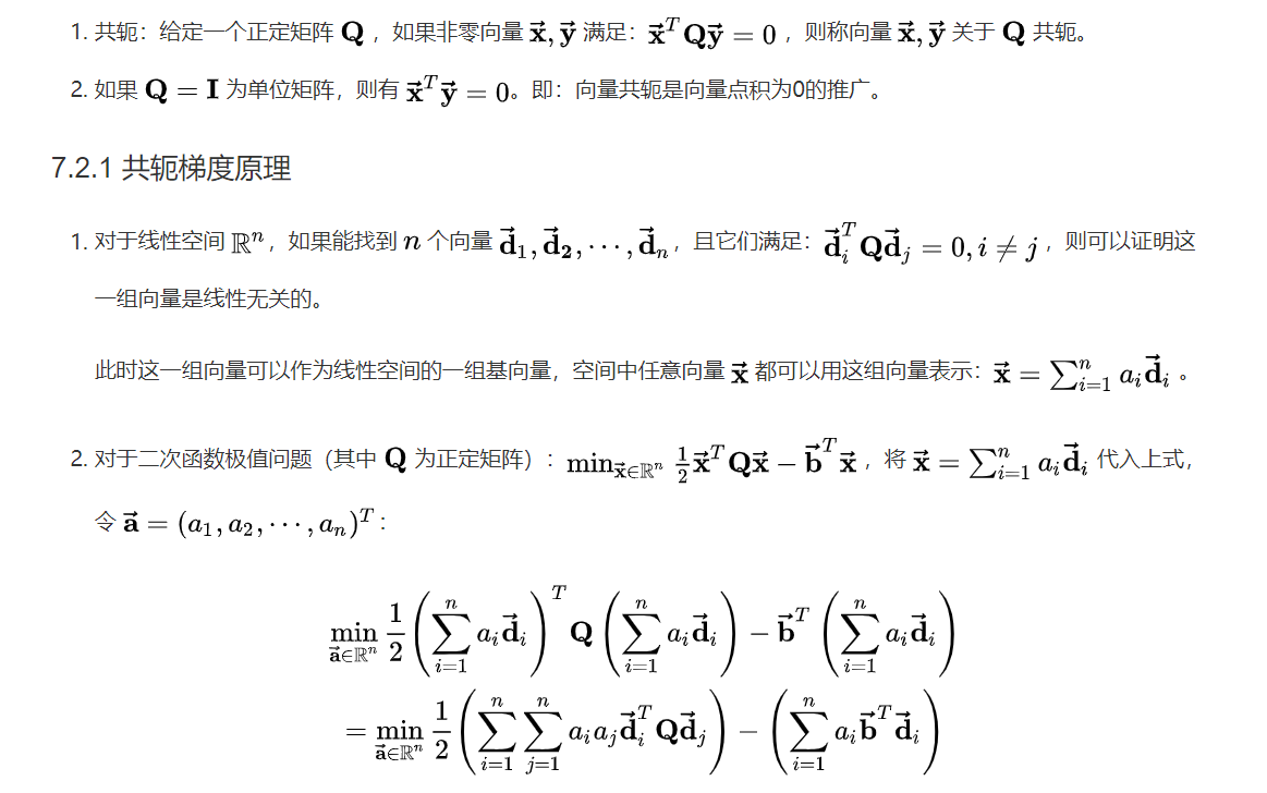
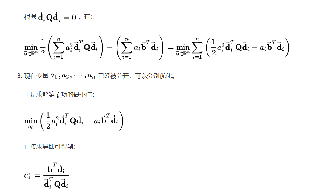
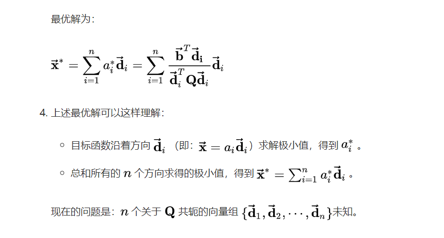
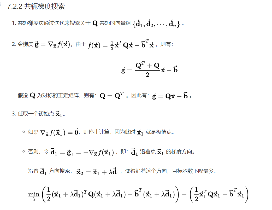
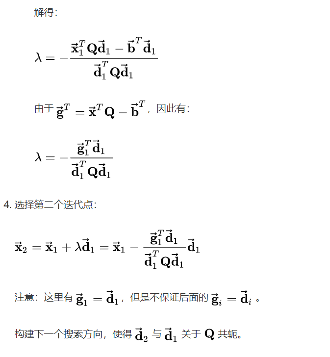
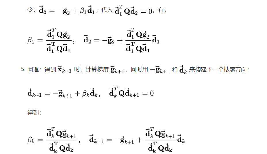
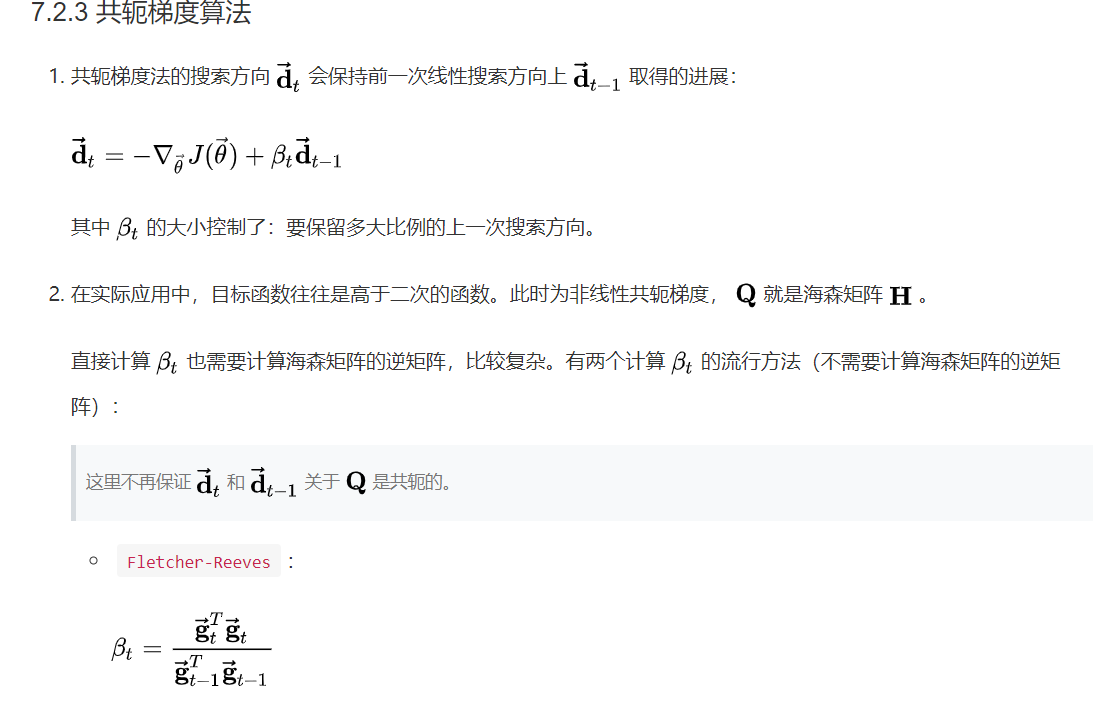
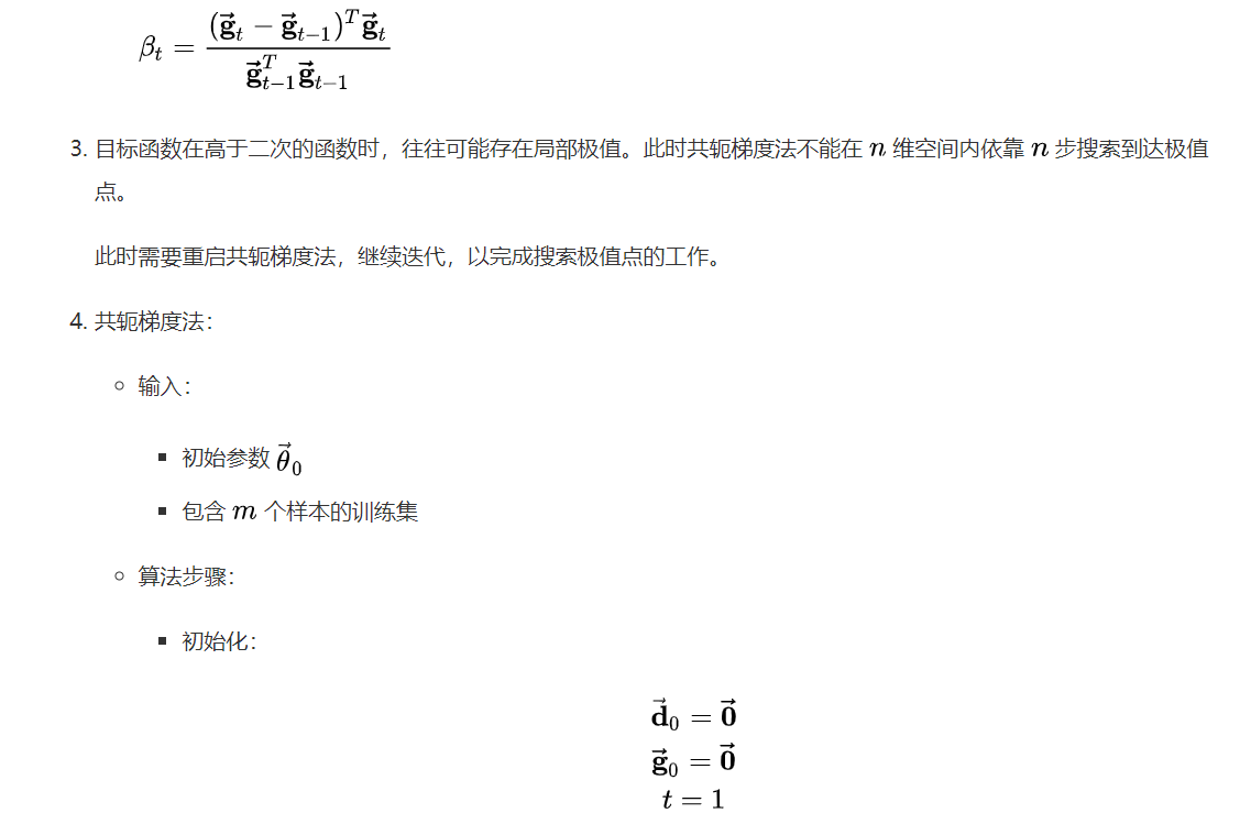
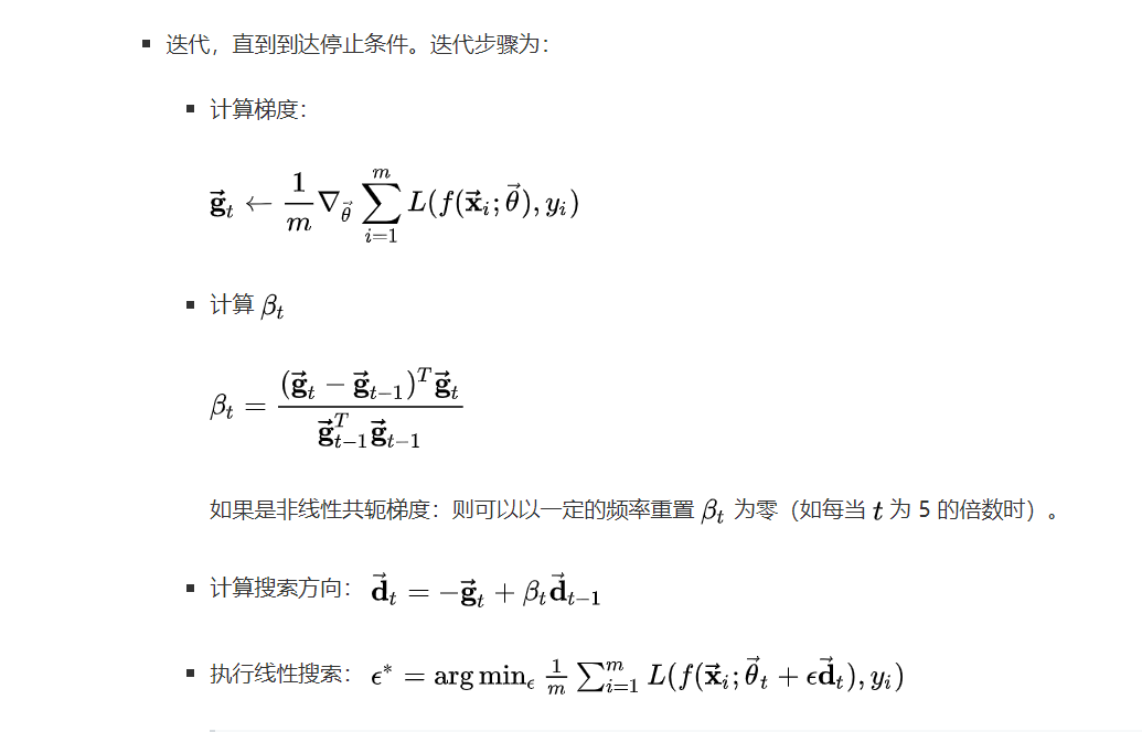
Combined with the above algorithm steps, I selected a two-dimensional function and compiled the program of conjugate gradient method for verification. The relevant programs are as follows:

from matplotlib import pyplot as plt
import numpy as np
import math

#The conjugate gradient method of positive definite quadratic function is also a kind of conjugate direction method. Its search direction is generated by the gradient at the minimum point obtained by one-dimensional search
#This program specifies a Function two-dimensional vector Function to test the algorithm and give the corresponding optimization results.

#Define objective function and partial derivative
def Function(x1,x2):
    value=3*math.pow(x1,2)+0.5*math.pow(x2,2)-x1*x2-2*x1
    return value
def Jac_x1(x1,x2):
    value=6*x1-2-x2
    return value
def Jac_x2(x1,x2):
    value=x2-x1
    return value

#Data initialization
X=[1,2] #Initial point k=0
x=[X[0],X[1]] #Keep a copy of the original point
Hessian=[[6,-1],[-1,1]] #Second order partial derivative matrix of objective function
Jac=[Jac_x1(X[0],X[1]),Jac_x2(X[0],X[1])] #Jacobian first order partial derivative vector
Direction=[-Jac[0],-Jac[1]]  #Initialize search direction
#Initialization step
Lambda=-(Jac[0]*Direction[0]+Jac[1]*Direction[1])/((Direction[0]*Hessian[0][0]+Direction[1]*Hessian[1][0])*Direction[0]+
        (Direction[0]*Hessian[0][1]+Direction[1]*Hessian[1][1])*Direction[1]) #Calculate the optimal step size lambda

X1=[X[0]+Lambda*Direction[0],X[1]+Lambda*Direction[1]] #Calculate next point
Jac1=[Jac_x1(X1[0],X1[1]),Jac_x2(X1[0],X1[1])]
Beta=(math.pow(Jac1[0],2)+math.pow(Jac1[1],2))/(math.pow(Jac[0],2)+math.pow(Jac[1],2)) #Initialize the value of Beta

#Setting accuracy
Epsilon=0.01

result=[]
Minimum=Function(X[0],X[1])
error=[]
count=0

while (math.sqrt(math.pow(Jac[0],2)+math.pow(Jac[1],2))>Epsilon):
    result.append(Function(X[0],X[1]))
    count+=1
    if(Function(X[0],X[1])<Minimum):
        Minimum=Function(X[0],X[1])
        
    #Update individual values
    X[0]=X1[0]
    X[1]=X1[1]
    #Update current Jacobian vector
    Jac=[Jac_x1(X[0],X[1]),Jac_x2(X[0],X[1])] 
    #Update search direction
    Direction=[-Jac[0],-Jac[1]] 
    #Update Lambda step value
    Lambda=-(Jac[0]*Direction[0]+Jac[1]*Direction[1])/((Direction[0]*Hessian[0][0]+Direction[1]*Hessian[1][0])*Direction[0]+
        (Direction[0]*Hessian[0][1]+Direction[1]*Hessian[1][1])*Direction[1])
    #Updates the next point of the current point
    X1=[X[0]+Lambda*Direction[0],X[1]+Lambda*Direction[1]]
    Jac1=[Jac_x1(X1[0],X1[1]),Jac_x2(X1[0],X1[1])]
    #Update beta value
    Beta=(math.pow(Jac1[0],2)+math.pow(Jac1[1],2))/(math.pow(Jac[0],2)+math.pow(Jac[1],2))

#Storage error
for i in range(0,count,1):
    error.append(result[i]-Minimum)
#Result analysis
print("The number of iterations is:{}".format(count))
print("The initial point is:({},{})The optimal value is:{}".format(x[0],x[1],Minimum))
print("The best advantages are:({},{})".format(X[0],X[1]))
plt.plot(result)
plt.title("The function value in the process of iteration")
plt.xlabel("The number of iteration")
plt.ylabel("The value of the function")
plt.figure()
plt.plot(error)
plt.title("The error in the process of iteration")
plt.xlabel("The number of iteration")
plt.ylabel("The value of error")
    

The running results of the program are shown below:

It can be seen that when we select the initial iteration point as (1, 2), the optimization value obtained by the final iteration of the algorithm is about - 0.4 and the number of iterations is 19. The change of function value in the iterative process is shown in the figure below:

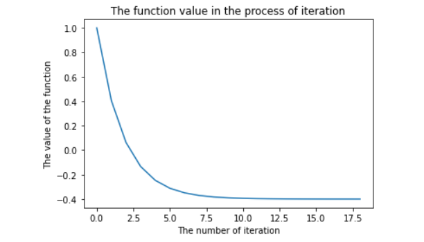
As can be seen from the above figure, the conjugate gradient algorithm can find the corresponding descent direction at a certain point and finally converge to an approximate optimal value. (if readers like, you can directly copy the program in this article and modify the accuracy, initial point and even function expression of the program to observe the impact of the algorithm on the iterative process)
The error variation of the algorithm is shown in the figure below:

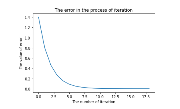
We can see that our error is also gradually decreasing, so the effect of our algorithm is still very good. Take action quickly! (programming)