Learn LBM calculation method for the first time, find an excellent example of flow around a cylinder written in python language, add notes to each code in detail to help you summarize, and provide some help for beginners (all the codes are at the end of the article).

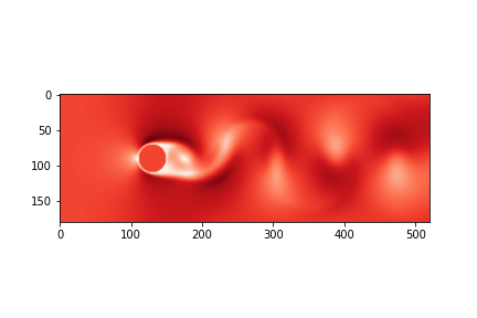
Put a result image first:

1. Import module, only two required

from numpy import *
from numpy.linalg import *
import matplotlib.pyplot as plt
from matplotlib import cm

2. Define the variables required by the LBM program:

maxIter = 200000 #Total calculation times
Re      = 100.0  #Reynolds number to be simulated by the model
nx = 520         #Model x-axis length
ny = 180         #Model y-axis length
ly=ny-1.0        #Later, it is used to calculate the inlet velocity and add disturbance to the model, because the calculation lacks disturbance when the Reynolds number is small.
q = 9            #Time D2Q9 model selected in this paper
cx = nx/4        #x coordinate of cylinder center
cy=ny/2          #y coordinate of cylinder center
r=ny/9           #Cylinder radius length
uLB = 0.04       #Inlet velocity of model
nulb=uLB*r/Re    #Viscosity coefficient of model fluid (radius is used here, strictly speaking, diameter should be used)
omega = 1.0 / (3.*nulb+0.5)  #Relaxation time of LBGK (single relaxation model)

It should be noted that the calculation of relaxation time (some say relaxation time, I'm not sure). To simulate the flow problem in LBM, you only need to control the same Reynolds number.

Reynolds number is:

In the flow around a cylinder, U represents the average inlet velocity, D represents the diameter of the cylinder, and v (nulb in the code) represents the fluid viscosity coefficient

In LBGK, the relationship between fluid viscosity coefficient and relaxation time is:

amongRepresents the relaxation time, c represents the lattice velocity (dx/dt), v represents the viscosity coefficient, and dt represents the time step

Through these two formulas, the velocity, Reynolds number, viscosity coefficient and relaxation time can be connected, which is convenient for the flexible regulation of model parameters in the future.

3. Define variables such as distribution function and lattice direction

#There are 9 directions represented by X and 2 directions represented by Y respectively
c = array([(x,y) for x in [0,-1,1] for y in [0,-1,1]])

#t represents the weight coefficient. The weight coefficient of N-S equation has three values: 1 / 36, 1 / 9 and 4 / 9
t = 1./36. * ones(q)            
t[asarray([norm(ci)<1.1 for ci in c])] = 1./9.
t[0] = 4./9.

#noslip is the opposite direction of lattice velocity
noslip = [c.tolist().index((-c[i]).tolist()) for i in range(q)] 

#i1 is 6, 7 and 8 directions, which is used for boundary treatment of exit boundary (right boundary)
i1 = arange(q)[asarray([ci[0]<0  for ci in c])] # Unknown on right wall.

#i2 is 0, 1 and 2 directions, which is used for boundary processing of entrance boundary (left boundary)
i2 = arange(q)[asarray([ci[0]==0 for ci in c])] # Vertical middle.

#i3 is 3, 4 and 5 directions, which is used for boundary treatment of entrance boundary (left boundary)
i3 = arange(q)[asarray([ci[0]>0  for ci in c])] # Unknown on left wall.

The grid direction number in this example is different from the general situation:

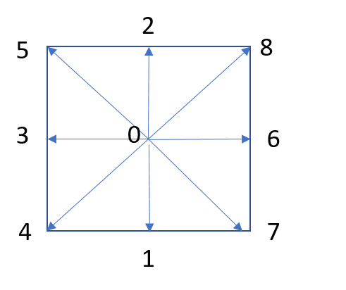
In fact, the direction can be determined according to the value of c. for example, the value of c[1] is [0, - 1], and the direction of its representative vector is [0, - 1], that is, along the negative direction of the y-axis.

4. Define the equation of equilibrium

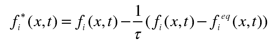
Collision and diffusion are basically similar to all LBM problems. Only the equilibrium equation determines the attribute of the problem, that is, the governing equation of the problem. The LBM equilibrium function under the N-S equation is expressed as:

The use code is expressed as:

sumpop = lambda fin: sum(fin,axis=0) #Define the function to calculate the macro density, and fin represents the particle distribution function

def equilibrium(rho,u):              #Equilibrium calculation

    cu   = 3.0 * dot(c,u.transpose(1,0,2))  #

    usqr = 3./2.*(u[0]**2+u[1]**2)

    feq = zeros((q,nx,ny))

    for i in range(q): feq[i,:,:] = rho*t[i]*(1.+cu[i]+0.5*cu[i]**2-usqr)

    return feq

What is more difficult to understand is the calculation of cu. Dot represents the dot product in numpy. The shape of c is (9,2), while the shape of u is (2, nx, ny). U. transfer (1,0,2), recorded as up, indicates that the first axis and the second axis are interchanged, and its shape becomes (nx,2,ny).

This is a multiplication of two-dimensional matrix and three-dimensional matrix. The result of the operation is that the shape of cu is (9,nx,ny)

The operation rules are complex and can be understood in combination with the physical meaning of lattice points:

First, c stays still. Starting from c[0], take out the first column of the first dimension of up, which is up[0,:,0]

c[0]*up[0,:,0] is equal to the first value of the first row of the first dimension of cu[0,0,0], that is, the value of the first grid point in the direction of 0

Then take out the second column of the first dimension of up, that is, up[0,:,1], c[0]*up[0,:,1] is equal to the second value of the first row of the first dimension of cu[0,0,1], that is, the value in the 0 direction of the second grid point

By analogy, all values of up can be obtained. Although the calculation is more abstract and requires more understanding and operation, it is much faster than its write loop to calculate.

5. Define cylinder correlation

obstacle = fromfunction(lambda x,y: (x-cx)**2+(y-cy)**2<r**2, (nx,ny))

#vel is used to initialize the speed. The value of d is 0, 1, which represents the x direction and y direction, and the value behind ulb represents the small deviation
#In fact, it doesn't matter to directly assign all values of 0.04
vel = fromfunction(lambda d,x,y: (1-d)*uLB*(1.0+1e-4*sin(y/ly*2*pi)),(2,nx,ny))

#Calculate the equilibrium state of all nodes
feq = equilibrium(1.0,vel)
#Initialize distribution function
fin = feq.copy()

It should be noted that numpy The function from function (f,shape) has two parameters. f function is used to build an array. Shape is the shape of the output of the array. The input of f function is related to shape, so the specific usage is not written.

obstacle is an array with the same shape as fin, in which the nodes outside the cylinder are false and the nodes inside the cylinder are true

vel is a variable that initializes the speed

6. Start calculation

for time in range(maxIter):

    #The outlet boundary condition, the fully developed flow scheme, that is, the unknown distribution function of the outlet is the same as the previous node
    fin[i1,-1,:] = fin[i1,-2,:] 
    
    rho = sumpop(fin)           #Calculate macro density
    
    u = dot(c.transpose(), fin.transpose((1,0,2)))/rho  #Calculate macro velocity

    #Entrance boundary condition, Zou he velocity boundary scheme
    u[:,0,:] =vel[:,0,:] 
    rho[0,:] = 1./(1.-u[0,0,:]) * (sumpop(fin[i2,0,:])+2.*sumpop(fin[i1,0,:]))
    
    #Calculated equilibrium state
    feq = equilibrium(rho,u)
    
    #Calculate the distribution function in 6, 7 and 8 directions of the inlet boundary
    fin[i3,0,:] = fin[i1,0,:] + feq[i3,0,:] - fin[i1,0,:]
    
    #Collision process
    fout = fin - omega * (fin - feq)
    
    #Applies a bounce format to nodes within a cylinder
    for i in range(q): fout[i,obstacle] = fin[noslip[i],obstacle]
    
    #diffusion process 
    for i in range(q):

        fin[i,:,:] = roll(roll(fout[i,:,:],c[i,0],axis=0),c[i,1],axis=1)
    
    #mapping
    if (time%10000==0):

        plt.clf(); plt.imshow(sqrt(u[0]**2+u[1]**2).transpose(),cmap=cm.Reds)

        plt.savefig("vel."+str(time/10000).zfill(4)+".png")

The highlight of the program. In LBM program design, in principle, it is OK to update the values of all nodes in the flow field. There is no strict sequence, but generally we follow the way of collision, diffusion and boundary treatment. However, this example is designed flexibly. Let's explain it in detail below:

According to the governing equation of LGBK:

After the particles complete a collision at the current node of the current time step, the particles in 8 directions will continue to reach the next node along 8 directions (the direction of 0 remains unchanged). For example, the particles in 6 directions (along the positive direction of X axis) at node (33, 33) will reach (33, 34),

Namely

When all nodes have completed the migration movement, the LBM calculation is completed at one time.

In this case, numpy is used The roll (a,shift,axis) function realizes the migration function. This function is used to scroll the array a forward along the axis axis (0 means along the column (y direction), 1 means along the row (x direction)), and the rolling interval is shift.

That is, when axis=0, row 0 becomes row 1, row 1 becomes row 2, and the last row becomes row 0. When axis=1, column 0 becomes column 1, column 1 becomes column 2, and the last column becomes column 0

In this example, the process of roll operation is that fout first scrolls a line forward along asix=0. At this time, it is equivalent to its x coordinate plus shift. The scrolling value should be c[i,0]. At this time, if i=6, 7, 8,c is positive, x coordinate plus 1, if c is 3, 4, 5,c is negative, x coordinate minus 1 Other directions are similar, and the second layer roll is also similar.  

This calculation is no problem for the upper and lower boundaries, because the particles going out of the upper boundary (directions 2, 5 and 8) roll and become the particles entering the lower boundary (Directions 1, 4 and 7), which is actually a periodic boundary condition in LBM. This boundary condition holds that the upper and lower boundaries are open and applicable to the calculation of flow around a cylinder (some also believe that the upper and lower boundaries are solid boundaries, so rebound boundary conditions need to be used)

However, there is a problem with the left and right boundaries. We know that the left and right boundaries are velocity boundary conditions, that is, the distribution function of the lattice points on the left boundary is calculated by Zou he boundary conditions. So we need to recalculate the value of the left and right boundaries at the beginning of the next cycle

In addition, for the treatment of cylindrical boundary, the direct rebound format is adopted in this example. We know that in the diffusion process, the particles of fluid node will enter the solid node in the direction of i, and the particles of solid node will enter the fluid node in the direction of - i. the rebound format is to reverse the direction of particles entering the solid node, After reversing, the particles in this direction will re-enter the fluid node in the next diffusion calculation.

The implementation method in this example is fout[i]=fin[noslip[i]]

So our calculation process of one cycle is:

• 1 - calculate the right boundary distribution function,
• 2 - calculate the macro density, macro velocity,
• Note that the density and velocity at the left boundary are wrong at this time, because the distribution function of the left boundary is migrated from the right boundary, but it doesn't matter, because the density (1.0) and velocity (0.04) of the left boundary are known quantities, so,
• 3 - recalculate the left boundary distribution function,
• At this time, we have performed an operation on all nodes, and then,
• 4 - calculate collisions for all nodes.
• 5 - dealing with cylindrical boundaries
• 6-diffusion calculation
• 7 - visualization

7. Model validation

The calculation results can be verified by the drag coefficient and lift coefficient. The calculation formula is:

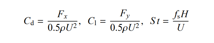
It has been tangled here for a long time. The main reason is the calculation of fx. The formula in some documents is:

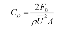
Here, Fd represents the total drag force and FX represents the drag force in the x direction. The difference between them is exactly one A (the two-dimensional case is the diameter of the circle). FX is relatively easy to obtain in LBM calculation, so we use the first formula.

The calculation of Fx adopts the momentum exchange method, and the specific calculation formula is:

Where s is the node in the solid and w is the node of the fluid adjacent to s.

python code is:

fx=0
fy=0

for i in range(q):

    for x in range(100,170,1): 

        for y in range(50,130,1):

            if obstacle[x,y]:

                x1=x+c[i,0]
                y1=y+c[i,1]

                if not obstacle[x1,y1]:

                    fx+=c[i,0]*(fout[i,x,y]+fout[noslip[i],x1,y1])
                    fy+=c[i,1]*(fout[i,x,y]+fout[noslip[i],x1,y1])


fx_1=abs(2*fx/(r*0.04**2))
fy_1=abs(2*fy/(r*0.04**2))

print(fx_1)
print(fy_1)

After 200000 calculations, the calculation takes about 2 hours, and the value of cd fluctuates around 3.2, which is in line with the calculation results in the literature. So far, the calculation of the flow around the cylinder is a complete success! Attach all codes:

# 2D flow around a cylinder
from numpy import *; from numpy.linalg import *
import matplotlib.pyplot as plt; from matplotlib import cm
###### Flow definition #########################################################
maxIter = 200000 # Total number of time iterations.
Re      = 220.0  # Reynolds number.
nx = 520; ny = 180; ly=ny-1.0; q = 9 # Lattice dimensions and populations.
cx = nx/4; cy=ny/2; r=ny/9;          # Coordinates of the cylinder.
uLB     = 0.04                       # Velocity in lattice units.
nulb    = uLB*r/Re; omega = 1.0 / (3.*nulb+0.5); # Relaxation parameter.

###### Lattice Constants #######################################################
c = array([(x,y) for x in [0,-1,1] for y in [0,-1,1]]) # Lattice velocities.
t = 1./36. * ones(q)                                   # Lattice weights.
t[asarray([norm(ci)<1.1 for ci in c])] = 1./9.; t[0] = 4./9.
noslip = [c.tolist().index((-c[i]).tolist()) for i in range(q)] 
i1 = arange(q)[asarray([ci[0]<0  for ci in c])] # Unknown on right wall.
i2 = arange(q)[asarray([ci[0]==0 for ci in c])] # Vertical middle.
i3 = arange(q)[asarray([ci[0]>0  for ci in c])] # Unknown on left wall.

###### Function Definitions ####################################################
sumpop = lambda fin: sum(fin,axis=0) # Helper function for density computation.
def equilibrium(rho,u):              # Equilibrium distribution function.
    cu   = 3.0 * dot(c,u.transpose(1,0,2))
    usqr = 3./2.*(u[0]**2+u[1]**2)
    feq = zeros((q,nx,ny))
    for i in range(q): feq[i,:,:] = rho*t[i]*(1.+cu[i]+0.5*cu[i]**2-usqr)
    return feq

###### Setup: cylindrical obstacle and velocity inlet with perturbation ########
obstacle = fromfunction(lambda x,y: (x-cx)**2+(y-cy)**2<r**2, (nx,ny))

#vel is used to initialize the speed. The value of d is 0, 1, which represents the x direction and y direction, and the value behind ulb represents the small deviation
#In fact, it doesn't matter to directly assign all values of 0.04
#vel = fromfunction(lambda d,x,y: (1-d)*uLB*(1.0+1e-4*sin(y/ly*2*pi)),(2,nx,ny))
vel = fromfunction(lambda d,x,y: (1-d)*uLB,(2,nx,ny))

feq = equilibrium(1.0,vel); fin = feq.copy()

w=zeros((9,nx,ny))
w[:,obstacle]=1


###### Main time loop ##########################################################
for time in range(maxIter):
    
    fin[i1,-1,:] = fin[i1,-2,:] #The outlet boundary condition, the fully developed flow scheme, that is, the unknown distribution function of the outlet is the same as the previous node
    
    rho = sumpop(fin)           #Calculate macro density
    
    u = dot(c.transpose(), fin.transpose((1,0,2)))/rho  #

    u[:,0,:] =vel[:,0,:] # 
    rho[0,:] = 1./(1.-u[0,0,:]) * (sumpop(fin[i2,0,:])+2.*sumpop(fin[i1,0,:]))

    feq = equilibrium(rho,u) # 
    fin[i3,0,:] = fin[i1,0,:] + feq[i3,0,:] - fin[i1,0,:]
    fout = fin - omega * (fin - feq)  # Collision process
    
    for i in range(q): fout[i,obstacle] = fin[noslip[i],obstacle]
    
    for i in range(q): #diffusion process 
        
        fin[i,:,:] = roll(roll(fout[i,:,:],c[i,0],axis=0),c[i,1],axis=1)
    
    if (time%2000==0): # Visualization

        fd=0
        ff=0

        for i in range(q):

            for x in range(100,170,1): 

                for y in range(50,130,1):

                    if obstacle[x,y]:

                        x1=x+c[i,0]
                        y1=y+c[i,1]

                        if not obstacle[x1,y1]:

                            fd+=c[i,0]*(fout[i,x,y]+fout[noslip[i],x1,y1])
                            ff+=c[i,1]*(fout[i,x,y]+fout[noslip[i],x1,y1])


        fd_1=abs(2*fd/(r*0.04**2))
        ff_1=abs(2*ff/(r*0.04**2))

        print(fd_1)
        print(ff_1)
            
    plt.clf(); plt.imshow(sqrt(u[0]**2+u[1]**2).transpose(),cmap=cm.Reds)
    plt.savefig("vel."+str(time/10000).zfill(4)+".png")