Detailed explanation of histogram back projection algorithm

concept

Back projection is a method to calculate the coincidence degree between pixels and pixels in the specified histogram model. In short, it is to first calculate the histogram model of a feature, and then use the model to find the feature in the image. For example, you have a hue saturation histogram, which you can use to find the skin color area in the image.

From the perspective of statistics, if the input histogram is regarded as a (a priori) probability distribution of a specific vector (color) on an object, the projection is to calculate the probability that a specified part of the picture comes from the a priori distribution (i.e. part of the object).

Set the original gray image matrix:

Image=
1 2 3 4
5 6 7 7
9 8 0 1
5 6 7 6
The gray value is divided into the following four intervals:
[0,2] [3,5] [6,7] [8,10]
It is easy to get the histogram of this image matrix hist = 4 462
Next, calculate the back projection matrix (the size of the back projection matrix is the same as that of the original gray image matrix):
The gray value with coordinate (0,0) in the original phase is 1,1, which is located in interval [0,2], and the histogram value corresponding to interval [0,2] is 4, so the value with coordinate (0,0) in the back projection matrix is recorded as 4. According to this method, the histogram direction projection matrix of image can be obtained by mapping in turn:
back_Projection=
4 4 4 4
4 6 6 6
2 2 4 4
4 6 6 6

What does the back projection of histogram represent?

In fact, the 256 gray values of the image are set to a few values. The specific values depend on how many intervals 0 ~ 255 are divided into (that is, how many bin)! The value of a point in the back projection is the gray histogram value of the interval where the point in the original image is located. Therefore, the more interval points, the brighter in the back projection matrix.
"Reverse" in back projection refers to the process of mapping from histogram value to back projection matrix.
Through back projection, the original image is simplified, and this simplified process is actually to extract a feature of the image. So we can use this feature to compare the two images. If the back projection matrices of the two images are similar or the same, we can judge that the feature of the two images is the same.

Code implementation based on OpenCV

First of all, the code refers to Mr. Jia Zhigang's original blog and adds some personal comments and understanding. Some of the code in the original blog is missing. After my digestion and understanding, I have completed the code.
Mr. Jia's original blog address: https://mp.weixin.qq.com/s/ZuMi66cK4lqM2VtbUhx9uQ

The codes described are as follows:

#include <opencv2/opencv. HPP > / / header file
#include <opencv2/highgui.hpp>
#include <iostream>
using namespace cv;
using namespace std;

//For 8-bit images, the closer this value is to 256, the more accurate the back projection effect will be, but the amount of calculation will also become larger But don't exceed 256, otherwise it doesn't make sense.
int bins = 64;

//This example deals with three channel RGB images
#define	 PROCESS_CHANNEL 3

//Set the images to be processed to be 8-bit. Reduce the dimension of the gray level of the image color to bins / pow (2,8) * pow (2,8), that is, bins
int gray_level = bins/pow(2,8)*pow(2, 8);
 

//OpenCV realizes LUT search through histogram interpolation without RGB color dimensionality reduction. My implementation goes the opposite way. I reduce the dimensionality of image color to obtain histogram, and no longer use LUT interpolation for histogram calculation.
void calculate_histogram(Mat &image, Mat &hist) 
{

	int width = image.cols;
	int height = image.rows;
	int r = 0, g = 0, b = 0;
	int index = 0;
	int level = 256 / bins;
	for (int row = 0; row < height; row++)
	{
		uchar* current = image.ptr<uchar>(row);
		for (int col = 0; col < width; col++)
		{
			if (image.channels() == 3) 
			{
				b = *current++;
				g = *current++;
				r = *current++;
				index = (r / level) + (g / level)*bins + (b / level)*bins*bins;
			}

			if (image.channels() == 1) 
			{
				r = *current++;
				index = (r / level);
			}
			hist.at<int>(index, 0)++;
		}
	}
}

int main(int argc, char *argv[])
{
	cv::Mat src = cv::imread("src.png", IMREAD_COLOR);
	cv::Mat model = cv::imread("model.png", 1);

	//If it's a single channel, gray_level is one-dimensional.
	//If it is three channels, the mixed histogram of three channels is three-dimensional. (the length, width and height are gray_level). Expand the three-dimensional into one dimension (the length is the third power of gray_level)
	gray_level = pow(gray_level, PROCESS_CHANNEL);

	//Model diagram
	Mat model_Hist = Mat::zeros(gray_level, 1, CV_32SC1);
	//Input diagram
	Mat src_Hist = Mat::zeros(gray_level, 1, CV_32SC1);

	if ( !model_Hist.data || !src_Hist.data)
	{
		printf("Image not found, please check the path\n");
		return -1;
	}
	cv::imshow("model", model);
	cv::imshow("src", src);

	//Calculate the histogram code of the input image and model as follows
	calculate_histogram(model, model_Hist);
	calculate_histogram(src, src_Hist);

	//Step 2: calculate the proportion R
	Mat ratio_hist = Mat::zeros(gray_level, 1, CV_32FC1);
	float m = 0, t = 0;

	for (int i = 0; i < gray_level; i++)
	{
		m = model_Hist.at<int>(i, 0);
		t = src_Hist.at<int>(i, 0);
		ratio_hist.at<float>(i, 0) = m / t;
	}

	//Step 3: calculate the probability distribution image
	// Find weight probability distribution (back projection)
	int r = 0, g = 0, b = 0;
	int level = pow(2,8) / bins;
	int index = 0;
	Mat w = Mat::zeros(src.size(), CV_32FC1);
	for (int row = 0; row < src.rows; row++) 
	{
		uchar* current = src.ptr<uchar>(row);
		for (int col = 0; col < src.cols; col++)
		{
			if (src.channels() == 3)
			{
				b = *current++;
				g = *current++;
				r = *current++;
				index = (r / level) + (g / level)*bins + (b / level)*bins*bins;
				w.at<float>(row, col) = ratio_hist.at<float>(index, 0);
			}
			else 
			{
				r = *current++;
				index = (r / level);
				w.at<float>(row, col) = ratio_hist.at<float>(index, 0);
			}
		}
	}

	//Step 4: convolution calculation In fact, the mean filtering is performed.
	Mat dst;
	Mat kernel = (Mat_<float>(3, 3) << 1, 1, 1,
									1, 1, 1,
									1, 1, 1);

	filter2D(w, dst, -1, kernel);//ddepth stands for "target depth", which is the depth of the result (target) image.
	//If you use - 1, the resulting (target) image will have the same depth as the input (source) image. The resulting (target) image will have the same depth as the input (source) image

	//Step 5: normalize and display the back projection results
	Mat result;
	normalize(dst, result, 0, 255, NORM_MINMAX);
	imshow("BackProjection Demo", result);


	
	cv::waitKey(0);
	return 0;
}

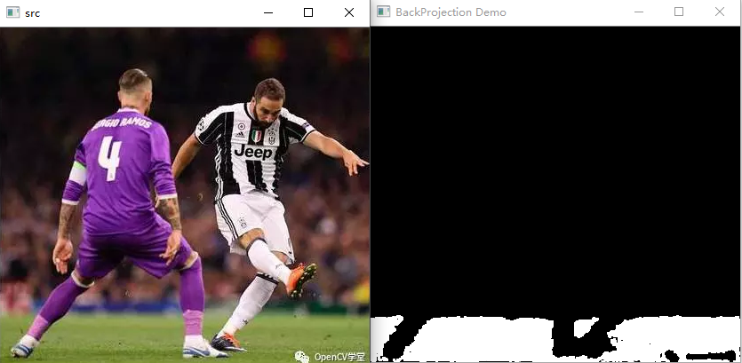
Code execution effect