Machine learning | R language | use random forest to evaluate the transaction price of second-hand cars

As a classification and regression algorithm to replace traditional machine learning methods such as neural network, random forest algorithm has the characteristics of high accuracy, not easy to over fit and high tolerance to noise and outliers. Compared with the traditional multiple linear regression model, random forest algorithm can overcome the complex interaction between covariates. [1] The random forest algorithm forms a forest by constructing multiple decision trees, and uses the bootstrap resampling method. The actual operation is to draw a certain number of samples from the original samples, and repeated sampling is allowed; Calculate the given statistics according to the extracted samples; Repeat the above steps several times to obtain a plurality of calculated statistics results; The statistical variance is obtained from the statistical results.

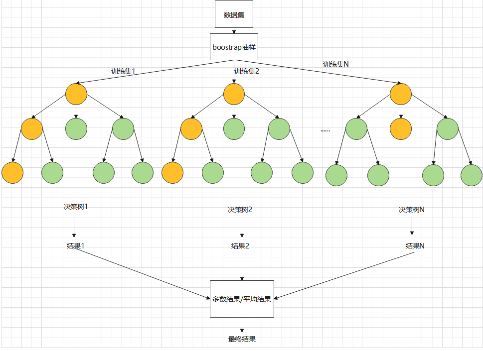
The process of random forest algorithm is as follows:

1. Assuming that the original sample size is N, bootstrap can be used to randomly select b self-help sample sets (the larger the sample size in the general sample set, the better the regression effect), so as to construct B regression trees. At the same time, the unselected data, that is, out of bag data (OOB), is used as the test sample of random forest;

2. Set the number of original data variables as p, randomly select a variable () at each node of each regression tree as the alternative branch variable, generally = p/3, and then select the optimal branch according to the branch optimality criterion (the same as the regression tree model); Among them, the branching optimality criterion is based on the sum of squares of mean deviation.

Suppose there are p independent variables and continuous dependent variable Y. In order to predict the second-hand car price, take the variables after data processing in Annex I as the independent variable X and the second-hand car transaction price as the continuous dependent variable Y.

For A node of the tree, the sample of t is {.. xn,yn}, and the sample size of the node is changed to N(t). Therefore, we can know the sum of squares of the deviation of the node. Assuming that all possible branch sets (including variables and corresponding tangent points) in this stage t are A, branch s divides node t into two child nodes and, in which the best branch is the branch with the largest difference between the sum of the square deviation of node t and the sum of the square deviation of the corresponding two child nodes after splitting, that is, the effect after splitting is better than that before splitting, The variation in each child node is minimized.

3. Each tree starts to branch recursively from top to bottom, sets the minimum size of leaf nodes as 5, and takes this as the termination condition for the growth of regression tree, that is, when the number of leaf nodes is less than 5, stop branching;

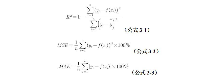
4. The generated b regression trees form a random forest regression model. The mean square error MSE, mean absolute error MAE and goodness of fit of out of pocket data (OOB) were used to evaluate the effect of regression. among

In this model, the ratio of training set to test level is 7:3.

previously on

With the development of China's economy, the automobile market is booming day by day. While the number of new cars is rising year by year, more consumers accept second-hand cars from the concept. In 2021, the trading volume of second-hand cars in China was 17.5851 million, up 22.6% from 14.3414 million in 2020. The increase of second-hand car trading volume has brought a larger second-hand car trading market, and also put forward higher requirements for the value evaluation of second-hand cars.
Nowadays, concepts and technologies such as big data, machine learning and in-depth learning have become increasingly popular and gradually began to be implemented to help enterprises reduce the cost of actual operation and production. In some countries with developed automobile industry (the United States, Japan, Germany, etc.), the use of big data technology to evaluate the transaction price of second-hand cars has been widely used in large enterprises, but big data technology has not been popularized in China. This paper establishes a prediction model based on random forest to evaluate the transaction price of second-hand cars.

data sources

The data used in this paper are from the data set attached to track A in the 2021 MathorCup college mathematical modeling challenge big data competition, with two annexes (Annex 1: Valuation training set and Annex 2: valuation verification set). There are 36 trains and 30000 lines in the training set, including 20 train information and market information such as vehicle series, manufacturer type, exhibition time and new car price. In addition, it also contains 15 columns of anonymous data, which does not give the specific meaning of the data. The last column is the exact transaction price of used cars. The data type of verification set is the same as that of training set, with A total of 10000 rows of data. We only use the data in Annex 1: training set in this article.

Import package and data reading:

###Import the required package
library(datasets)
library(plyr)
library(randomForest)
library(xlsx)
require(caret)
library(ggplot2)
library(vioplot)
library(dplyr)
library(tidyverse)
###Data reading
set.seed(987654321)	#Set random seed
data <- read.csv('F:/R/Processing data.csv')
data <- data[,c(-1,-2)]	#Since the first two columns of the data set are the data table with serial number and vehicle id, they are useless information, so they are deleted

Data preprocessing

Data completion and variable deletion

Firstly, the training set and verification set in Annex 1 and Annex 2 are preprocessed. The data processing methods of Annex I and Annex II are the same. Analyze the number of missing values in each data. The number of missing items is as follows:

Missing variable name	Annex 1: Valuation training data
country	3757
maketype	3641
modelyear	312
carCode	9
gearbox	1
anonymousFeature1	1582
anonymousFeature4	12108
anonymousFeature7	18044
anonymousFeature8	3775
anonymousFeature9	3744
anonymousFeature10	6241
anonymousFeature11	461
anonymousFeature12	0
anonymousFeature13	1619
anonymousFeature15	27580

According to the analysis of the number of missing variables, there are the processing methods in the following table:

variable	Treatment method
country	Mode completion
maketype
modelyear
carcode
anonymousFeature8
anonymousFeature9
anonymousFeature10
anonymousFeature1	Delete variable
anonymousFeature4
anonymousFeature7
anonymousFeature15
anonymousFeature13
tradeTime	Calculate the difference to construct a new variable
licenseDate	Calculate the difference to construct a new variable
anonymousFeature12	After splitting into three variables, the missing value is supplemented by mode
anonymousFeature11	Special value substitution

Where country is the country, maketype is the manufacturer type, modelyear is the model year, carcode is the national standard code, and gearbox is the gearbox, which can be regarded as sub type data, and the mode of its corresponding data is used to complete. It should be noted that since the amount of data in Annex 2 is far less than that in Annex 1, the missing data in the verification set of Annex 2 are supplemented with the mode of the data corresponding to Annex 1, so as to ensure more rationality.

Anonymous variable 8, anonymous variable 9 and anonymous variable 10 only have several possible values, which can also be regarded as typed data and supplemented by mode. Analyzing the original data, it is found that the data value of anonymous variable 1 is all 1, the variance is 0, and there is no amount of information, so it is eliminated. Anonymous variable 4, anonymous variable 7 and anonymous variable 15 contain a large number of missing values and only a small number of valid values, so they are eliminated. Anonymous 13 and license date are similar to the registration date. In order to avoid repeated use of data and increase workload, anonymous 13 and license date are excluded.

Considering that the use time of second-hand cars has a great impact on the price of second-hand cars, a new variable is constructed by subtracting the registration date from the exhibition date: the use days of second-hand cars. Because the exhibition date and year are the same, the variance is 0, so it is excluded. In addition, the year of registration date shall be retained, and the month and date data with less impact shall be excluded.

Anonymous variable 11 has 1, 1 + 2, 3 + 2, (1 + 2, 4 + 2) and other types, which can also be regarded as typed data. The values 1, 2, 3 and 4 are used to represent these four types respectively, and the mode is taken for completion. Anonymous variable 12 is in the form of multiplying three multipliers, which is guessed as length, width and height, multiplied by physical quantities such as the volume of the vehicle. Therefore, the three multipliers are divided into three columns of data to form three new variables, so as to enhance the integrity of the data and finally form the data set used in the project.

Data preprocessing script code (python):

import pandas as pd
from pandas import read_csv

# Listing
names = ['carid', 'tradeTime', 'brand', 'serial', 'model', 'mileage', 'color', 'cityId', 'carCode', 'transferCount',
         'seatings',
         'registerDate', 'licenseDate', 'country', 'maketype', 'modelyear', 'displacement', 'gearbox', 'oiltype',
         'newprice']

# Fill the column name
modenames = ['country', 'maketype', 'modelyear', 'carCode', 'gearbox', 'anonymousFeature1'
    , 'anonymousFeature8', 'anonymousFeature9', 'anonymousFeature10']

# Delete column name
delete_name = ['anonymousFeature4', 'anonymousFeature7', 'anonymousFeature15', 'tradeTime'
    , 'registerDate', 'licenseDate', 'anonymousFeature12', 'anonymousFeature13', 'anonymousFeature1']

# Record the corresponding mode
modedict = {}

# Fill mode
def fillmode(train, name):
    mod = train[name].mode()
    mod = mod.tolist()[0]
    train[name].fillna(mod, inplace=True)
    x = {name: mod}
    modedict.update(x)

# Split data processing
def sepdata(train):
    # # Time processing
    train['tradeTime'] = pd.to_datetime(train['tradeTime'])
    train['registerDate'] = pd.to_datetime(train['registerDate'])
    train['licenseDate'] = pd.to_datetime(train['licenseDate'])

    train['registerDate_year'] = train['registerDate'].dt.year
    train['used_time'] = train['tradeTime'] - train['licenseDate']
    train['used_time'] = train['used_time'].dt.days

    # Segmentation processing
    res = train['anonymousFeature12'].str.split('*', expand=True)
    train['length'] = res[0]
    train['width'] = res[1]
    train['high'] = res[2]

    # Segmentation processing
    train['anonymousFeature11'] = train['anonymousFeature11'].map(func)

# Anonymous variable mapping
def func(x):
    if x == '1':
        x = 1
    elif x == '1+2':
        x = 2
    elif x == '3+2':
        x = 3
    else:
        x = 4
    return x

# Processing process
def process(train, filename):
    sepdata(train)
    for name in names:
        if name in modenames:
            fillmode(train, name)
        if name in delete_name:
            train = train.drop(name, 1)
    print(train)
    # Add length width height mode
    modedict.update({'length': train['length'].mode().tolist()[0]})
    modedict.update({'width': train['width'].mode().tolist()[0]})
    modedict.update({'high': train['high'].mode().tolist()[0]})
    train.to_csv(filename)

# Process validation data
def process_eval(eval, filename):
    sepdata(eval)
    for name in names:
        # Fill in Annex I mode
        if name in modedict.keys():
            eval[name].fillna(modedict[name], inplace=True)
        if name in delete_name or name == 'price':
            eval = eval.drop(name, 1)

    eval['width'].fillna(modedict['width'], inplace=True)
    eval['high'].fillna(modedict['width'], inplace=True)
    eval['length'].fillna(modedict['width'], inplace=True)
    print(eval)
    eval.to_csv(filename)

if __name__ == "__main__":
    for i in range(15):
        names.append('anonymousFeature' + str(i + 1))
    names.append('price')

    train = read_csv('enclosure/Annex 1: Valuation training data.csv', sep='\t', names=names)
    process(train, './enclosure/Processing data 1.csv')

    eval = read_csv('enclosure/Annex 2: appraisal verification data.csv', sep='\t', names=names)
    process_eval(eval, './enclosure/Validation data.csv')

Data outlier handling

After the preliminary processing of the data, the points with obvious errors in the given data need to be handled abnormally. In this paper, the box diagram method is mainly used to process the abnormal data. Box chart is a statistical chart used to represent the dispersion of data, which mainly reflects the distribution characteristics of data.
There are mainly five points in the box chart, which are called upper limit, lower limit, Q3 (upper quartile, i.e. the number of positions), Q2 (median) and Q1 (lower quartile, i.e. the number of positions). The upper limit is equal to Q3+1.5IQR, the lower limit is equal to Q1-1.5IQR, and there is IQR=Q3-Q1. When the data exceeds the upper and lower limits of the corresponding box chart, it can be judged as an abnormal value. The schematic diagram is as follows:

Remove outliers:

OutVals = boxplot(data[,'price'], plot=FALSE)$out
data <- data[-(which(data[,'price'] %in% OutVals)),]	#Remove data rows with abnormal price value
data <- data[-(which(data[,'country']==0)),]	#Some country values are 0, belonging to the category of outliers

We remove outliers, and establish random forest models before and after removing outliers to compare their performance. (except for the row where the outlier is located, other data are the same, and all parameters of the random forest adopt the default parameters). The results are as follows:

	Before outlier removal	After outliers are removed
R square	0.000266	0.934676

It can be seen that the performance of the model has been greatly improved after removing outliers, so this step is very critical.

Establishment and optimization of Stochastic Forest Model

Tree selection

In this project, we adjust three important parameters of random forest, such as ntree, mtry and maxdepth. First, we adjust ntree, that is, the number of decision trees in random forest.
We use the preprocessed data, and the parameters of random forest are set as the default:

train_sub <- sample(datasize,round(0.7*datasize))	#Scramble data sets
train_data <- data[train_sub,]
test_data <- data[-train_sub,]	#The original data set is randomly divided into training set and verification set according to the ratio of 7:3

fit.rf1 <- randomForest(price~. ,data=train_data,importance=T)	#Generating random forest prediction model
plot(fit.rf1)	#plot() function is used to draw the curve of the prediction error of random forest with the number of decision trees

Get the following figure:

It can be seen from the figure that when the number of decision trees in the random forest exceeds 500, the error of the random forest is basically unchanged. In order to make the model more efficient and shorten the training time of the model, we determine the number of decision trees as 500.

Selection of independent variables

After establishing the preliminary random forest model (using the default parameters), it is also necessary to adjust the number of independent variables accordingly, so as to obtain the best R2 value and optimize the accuracy of the model.

train_sub <- sample(datasize,round(0.7*datasize))
train_data <- data[train_sub,]
test_data <- data[-train_sub,]	#Obtain training set and verification set

fit.rf <- randomForest(price~. ,data=train_data,importance=T)	#If the importance is set to T, the random forest can be used to calculate the importance of each variable
im <- importance(fit.rf,type=2)	#Save results
pred <- predict(fit.rf,test_data)
obs <- test_data[,'price']
result <- data.frame(obs,pred)
obs <- as.numeric(as.character(result[,'obs']))
pred <- as.numeric(as.character(result[,'pred']))
r <- r2fun(pred,obs)	#Calculate the R2 of the model and judge the performance of the model according to this standard
print(im)	#Ranking of importance of output independent variables

The importance ranking of each variable when the variable is not deleted at first:

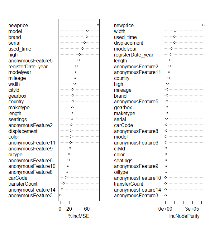
Next, we will start with the variables with the lowest importance and delete the variables with a large difference in importance from other variables. After deleting each variable, recalculate the importance ranking of each variable and repeat the above operation. Three variables were deleted and four experiments were conducted for horizontal comparison:

arrange mode	R2
Do not delete	0.932
Delete four variables anonymousFeature14 anonymousFeature10 anonymousFeature9 anonymousFeature3	0.935
Delete nine variables anonymousFeature14,anonymousFeature10,anonymousFeature9,anonymousFeature3,color,transferCount,oiltype,cityId,seatings	0.942
Delete eleven variables anonymousFeature14,anonymousFeature10,anonymousFeature9,anonymousFeature3,color,transferCount,oiltype,cityId,seatings anonymousFeature8,carCode	0.929

It can be seen that after eleven variables are deleted, MSE starts to decrease, so it is not suitable to delete too many variables. Finally, brand (brand id), serial (vehicle id), model (model id), mileage (mileage), cityId (City id), carCode (National Standard Code), country (country), maketype (manufacturer type), model year (model year), displacement (displacement) are selected for this model, gearbox, oiltype, newprice, anonymousFeature2, anonymousFeature5, anonymousFeature6, anonymousFeature8, anonymousFeature11, registerDate_year, used_time, length, width and height are 23 variables to construct the corresponding random forest model.

Adjustment of mtry parameters

Mtry represents how many independent variables are randomly selected from all independent variables for the establishment of each decision tree. For example, when the mtry value is 5, if we take 13 independent variables to establish a random forest, then 5 independent variables will be randomly selected from the 13 independent variables as the classification standard when each decision tree is established.
For the parameter adjustment of mtry, we use the traversal method to traverse all mtry parameters within a reasonable range, and take the mtry parameter value when the model result is the best.
We have 21 independent variables, so we set the range of mtry to (2:20), because the value of mtry cannot be less than 2 or greater than or equal to the total number of independent variables.
mtry parameter adjustment Code:

###mtry parameter adjustment
r2list <- c()	#r2list is used to record the R2 value of the model determined by each different mtry value, so as to judge the performance of the model
r2best <- 0	#It is used to store the maximum R2 value, that is, the best model performance value
mtrybest <- 0	#Record the corresponding value of mtry when the model performance reaches the best
r_m <- 0	
for(i in 2:20)
{
  fit.rf1 <- randomForest(price~. ,data=train_data1,importance=T,proximity=TRUE,ntree=500,mtry=i)
  pred1 <- predict(fit.rf1,test_data1)
  obs1 <- test_data1[,'price']
  result1 <- data.frame(obs1,pred1)
  obs1 <- as.numeric(as.character(result1[,'obs1']))
  pred1 <- as.numeric(as.character(result1[,'pred1']))
  
  r_m <- r2fun(pred1,obs1)
  r2list <- c(r2list,r_m)
  if( r_m > r2best)	#If the R2 value of the current model is r_ If M is larger than the value stored in r2best, replace the value of r2best with r_m
  {
    r2best <- r_m
    mtrybest <- i
  }
  
}

If you want to draw the curve of R2 changing with mtry parameter, just add the following code:

plot(x=c(2:20),y=r2list,xlab='mtry',ylab='R2',main='R2 along with mtry Value change diagram')

Here we will not show them one by one.
The final optimal R2 value and corresponding mtry value are shown in the table below:

evaluating indicator	R square	MSE	MAE
Test set	0.9541	1.8406	0.8649

maxdepth parameter

The adjustment process of maxdepth parameter is basically the same as that of mtry. Set the range as seq (10100,10), that is, between 10 and 100, and take 10 as the span value.
maxdepth parameter code:

###maxdepth parameter
r2list <- c()	#Record R2 corresponding to different maxdepth values
r2best <- 0	#Record the maximum value of R2
maxdepthbest <- 0	#Record the maxdepth value corresponding to the maximum R2
r_d <- 0
for(j in seq(10,100,10))
{
  fit.rfd <- randomForest(price~. ,data=train_data,importance=T,proximity=TRUE,ntree=500,mtry=20,max_depth=j)
  pred <- predict(fit.rfd,test_data)
  obs <- test_data[,'price']
  result <- data.frame(obs,pred)
  obs <- as.numeric(as.character(result[,'obs']))
  pred <- as.numeric(as.character(result[,'pred']))
  
  
  r_d <- r2fun(pred,obs)
  depthlist <- c(depthlist,r_d)
  if( r_d > r2best)
  {
    r2best <- r_d
    maxdepthbest <- j
  }
}

The principle is the same as the parameter adjustment process of mtry. Due to the time relationship, we did not calculate the final result in the end. Because of the large amount of data, the construction time of the model is long, and our time for this project is limited. Interested partners can try oh.

Extended article

GridSearch method

The above method we use to adjust the parameters of mtry and maxdepth is to first find the best value of mtry, then fix it, and then adjust the parameters of maxdepth. Although this method is faster than GridSearch, it is easy to fall into local optimization.

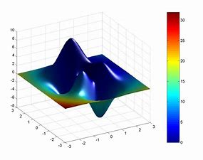
Like this picture, we may reach the peak of a small peak, but it is not the highest vertex in the whole surface. In this case, we only reach the local optimum, not the global optimum. To achieve global optimization, we can use GridSearch method.
So what is GridSearch? The Chinese literal translation of GridSearch is grid search. This sounds very tall, but in fact, the principle is very simple. It is to nest the traversal loops of different parameters to get the optimal combination of parameters. Don't say much, let's start with the code:

###GridSearch method
r2list <- c()	#Record R2 corresponding to different parameter combinations of maxdepth and mtry
r2best <- 0	#Record the maximum value of R2
mtrybest <- 0    #Record the corresponding value of mtry when R2 is maximum
depthbest <- 0    #Record the corresponding value of depth when R2 is maximum
r_g <- 0    
for(i in 2:20)
{
  for(j in seq(10,100,10))
  {
    fit.rf1 <- randomForest(price~. ,data=train_data1,importance=T,proximity=TRUE,ntree=500,mtry=i,maxdepth=j)
    pred1 <- predict(fit.rf1,test_data1)
    obs1 <- test_data1[,'price']
    result1 <- data.frame(obs1,pred1)
    obs1 <- as.numeric(as.character(result1[,'obs1']))
    pred1 <- as.numeric(as.character(result1[,'pred1']))
    
    r_g <- r2fun(pred1,obs1)
    r2list <- c(r2list,r_m)
    
    if( r_g > r2best)    
    {
      r2best <- r_g
      mtrybest <- i
      depthbest <- j
    }
  }
}

It can be seen that there is no essential change in this method. It is also traversal to find the optimal parameters. But it is no longer the traversal of a single parameter, but the traversal of a combination of two parameters. If there are 19 cases of mtry and 10 cases of maxdepth in this project, there are 190 cases of their parameter combination. These 190 situations are like many small grids on a large Internet. Grid search is to find the small grid that makes R2 the largest among the 190 small grids, that is, the best parameter combination of mtry and maxdepth. In this way, the global optimization can be achieved naturally, but at the same time, the amount of calculation is also greatly increased. Due to the limited computing power of our equipment, we did not adopt the GridSearch method. Interested partners can try it.

Cross validation

Cross validation refers to dividing the data set into k parts, which are used as the validation set in turn, and the other (k-1) data sets are used as the training set. Finally, K models are obtained, and the results of these K models are averaged during regression analysis, which will make the predicted value more stable and accurate.
Attach cross validation code:

###Cross validation
CVgroup <- function(k,datasize,seed){
  cvlist <- list()
  set.seed(seed)
  n <- rep(1:k,ceiling(datasize/k))[1:datasize]    #Divide the data into K parts and generate data set n
  temp <- sample(n,datasize)   #Disrupt n
  x <- 1:k
  dataseq <- 1:datasize
  cvlist <- lapply(x,function(x) dataseq[temp==x])  #Randomly generate k randomly ordered data columns in dataseq
  return(cvlist)
}

K is the number of subsets divided, datasize is the size of the dataset, and seed is the random seed set by yourself. Divided into k parts is k-fold cross validation.
This project can also use k-fold cross validation. However, due to the limited computing power and time of the equipment, we did not adopt the cross validation method. Interested partners can try it by themselves.

Topics: Python R Language

Programmer Think