Recently, I have worked hard to find resource animation to summarize the classic sorting algorithm. Some animations have not been found yet, but I will continue to update them later, which is suitable for beginners.
Overview of sorting algorithm
Sorting: adjust a group of "unordered" record sequences to "ordered" record sequences.
List sorting: change an unordered list into a sequential table.
Input: List
Output: ordered list
Ascending and descending order
Built in sorting function: sort()
Outline of sorting method:
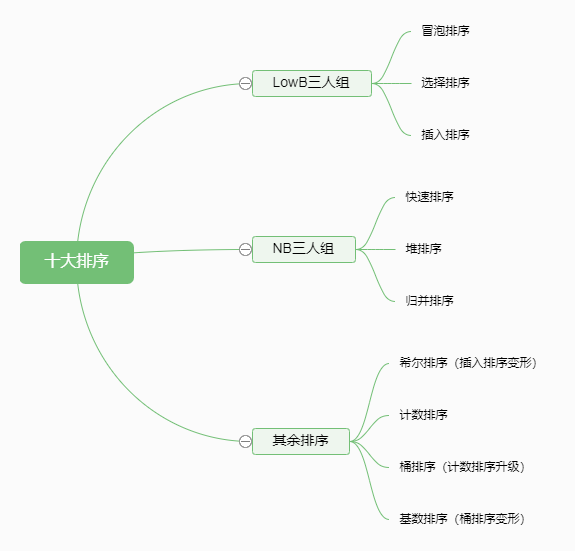
The following is the arrangement
| Sorting algorithm | Average time complexity | Best case | Worst case scenario | Spatial complexity | stability |
|---|---|---|---|---|---|
| Bubble sorting | O ( n 2 ) O(n^2) O(n2) | O ( n ) O(n) O(n) | O ( n 2 ) O(n^2) O(n2) | O ( 1 ) O(1) O(1) | stable |
| Select sort | O ( n 2 ) O(n^2) O(n2) | O ( n 2 ) O(n^2) O(n2) | O ( n 2 ) O(n^2) O(n2) | O ( 1 ) O(1) O(1) | instable |
| Insert sort | O ( n 2 ) O(n^2) O(n2) | O ( n ) O(n) O(n) | O ( n 2 ) O(n^2) O(n2) | O ( n ) O(n) O(n) | stable |
| Quick sort | O ( n l o g n ) O(nlogn) O(nlogn) | O ( n l o g n ) O(nlogn) O(nlogn) | O ( n 2 ) O(n^2) O(n2) | O ( n l o g n ) O(nlogn) O(nlogn) | instable |
| Heap sort | O ( n l o g n ) O(nlogn) O(nlogn) | O ( n l o g n ) O(nlogn) O(nlogn) | O ( n l o g n ) O(nlogn) O(nlogn) | O ( 1 ) O(1) O(1) | instable |
| Merge sort | O ( n l o g n ) O(nlogn) O(nlogn) | O ( n l o g n ) O(nlogn) O(nlogn) | O ( n l o g n ) O(nlogn) O(nlogn) | O ( n ) O(n) O(n) | stable |
| Shell Sort | O ( n l o g n ) O(nlogn) O(nlogn) | O ( n l o g 2 n ) O(nlog^2n) O(nlog2n) | O ( n l o g 2 n ) O(nlog^2n) O(nlog2n) | O ( 1 ) O(1) O(1) | instable |
| Count sort | O ( n + k ) O(n+k) O(n+k) | O ( n + k ) O(n+k) O(n+k) | O ( n + k ) O(n+k) O(n+k) | O ( k ) O(k) O(k) | stable |
| Bucket sorting | O ( n + k ) O(n+k) O(n+k) | O ( n + k ) O(n+k) O(n+k) | O ( n 2 k ) O(n^2k) O(n2k) | O ( n k ) O(nk) O(nk) | stable |
| Cardinality sort | O ( k n ) O(kn) O(kn) | O ( k n ) O(kn) O(kn) | O ( k n ) O(kn) O(kn) | O ( n + k ) O(n+k) O(n+k) | stable |
Note: the stability of sorting algorithm refers to that the relative position of the same elements before and after sorting remains unchanged, so the sorting algorithm is stable; Otherwise, the sorting algorithm is unstable.
Let's start with the implementation of various algorithms. The routines are sorted from small to large.
1. Bubble sorting
Principle: it repeatedly visits the sequence to be sorted, compares two elements at a time, and exchanges them if they are in the wrong order. Float the smallest number up, or sink the largest data.
Every two adjacent numbers in the list. If the front is larger than the back, exchange these two numbers. After a sequence is completed, the disordered area will be reduced by one number and the ordered area will be increased by one number.

def bubble_sort(lis):
    for i in range(len(lis)-1):
        exchange = False
        for j in range(len(lis)-i-1):
            if lis[j] > lis[j+1]:
                lis[j], lis[j+1] = lis[j+1], lis[j]
                exchange = True

        if not exchange: # If the order is arranged, that is, you do not need to continue sorting at one time, return directly
            return
	return

lis = [3,2,1,4,5]
bubble_sort(lis)
print(lis)
2. Select Sorting
Principle: selective sorting is very similar to bubbling. It also compares two elements, but it does not exchange until the largest or smallest data is selected.
The minimum number of records in one pass sorting is placed in the first position, and the minimum number in the disordered area of the record list in one pass sorting is placed in the second position.

def select_sort(lis):
    for i in range(len(lis)-1):
        min_num = i
        for j in range(i+1, len(lis)):
            if lis[min_num] > lis[j]:
                min_num = j
        if min_num != i:
            lis[i], lis[min_num] = lis[min_num], lis[i]
    return

lis = [3,2,5,4,6,8]
print(lis)
select_sort(lis)
print(lis)
3. Insert sort
Principle: starting from the second data, the current number (the first trip is the second digit) is compared with the previous number in turn. If the previous number is greater than the current number, the number will be placed at the position of the current number, and the subscript of the current number is - 1 until the current number is not greater than a previous number. Until the last element is traversed.
Generally speaking, starting from the second place, insert smaller values forward. The previous data must be the position where the insertion sort has been arranged, and the previous value is less than or equal to the benchmark value of the current value.
At the beginning, there is only one card in the hand (ordered area). Touch one card every time (from the disordered area) and insert it into the correct position of the existing card in the hand.

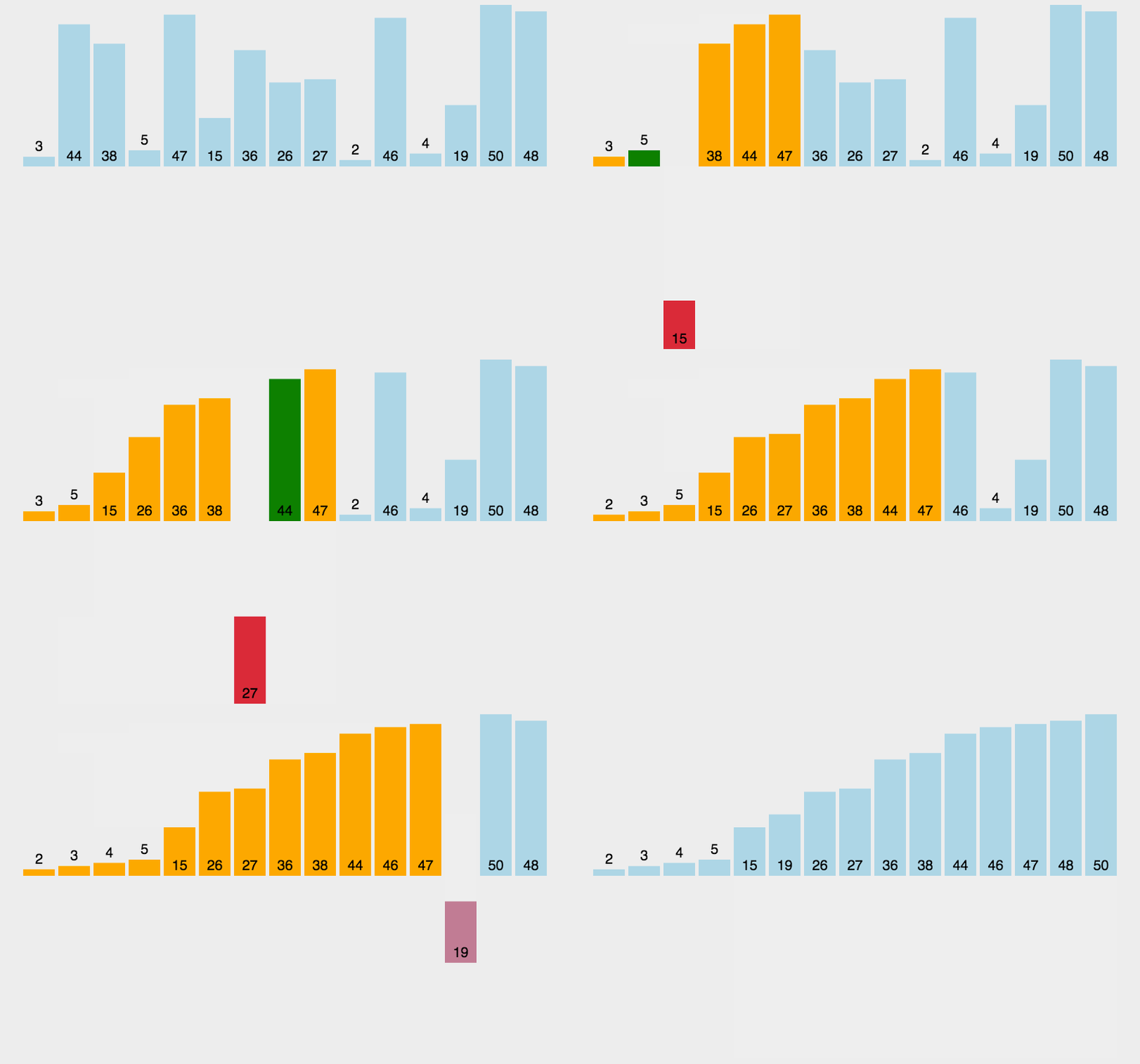
The Python code is implemented as follows:
def insert_sort(lis):
    for i in range(1, len(lis)):
        temp = lis[i] # Touched cards
        j = i - 1  # It refers to the cards in your hand
        while lis[j] > temp and j >= 0:
            lis[j+1] = lis[j]
            j -= 1
        lis[j+1] = temp

lis = [3,2,4,1,5]
insert_sort(lis)
print(lis)
4. Quick sort
Principle: divide the sequence into left and right parts through one-time sorting, in which the value of the left part is smaller than that of the right part, and then sort the records of the left and right parts respectively until the whole sequence is in order.
Quick sorting idea:
- Take an element p (the first element) and make element p belong to;
- The list is divided into two parts by P, the left is smaller than P, and the right is larger than p;
- Sort recursively.
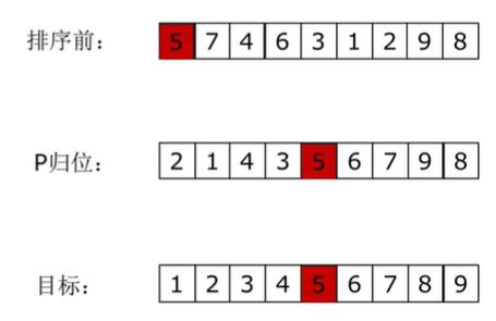

The Python code is implemented as follows:
def quick_sort(lis, left, right):
    if left < right:
        mid = partition(lis, left, right)
        quick_sort(lis, left, mid-1)
        quick_sort(lis, mid+1, right)

def partition(lis, left, right):
    temp = lis[left]
    while left < right:
        while left < right and lis[right] >= temp:
            right -= 1
        lis[left] = lis[right]
        while left < right and lis[left] <= temp:
            left += 1
        lis[right] = lis[left]
    lis[left] = temp
    return left

lis = [3,5,2,5,6,7,1]
quick_sort(lis, 0, len(lis)-1)
print(lis)
5. Heap sorting
Heap sort is a sort algorithm designed by using the data structure of heap. A general property of heap is used, that is, the key value or index of a child node is always less than (or greater than) its parent node.
Content supplement:
A tree is a data structure, such as a directory structure
A tree is a data structure that can be defined recursively
Number is a set of n nodes:
- If n=0, then this is an empty tree;
- If n > 0, there is one node as the root node of the number, other nodes can be divided into m combinations, and each set itself is a tree.
Some concepts:
- Root node; Leaf node (no more points)
- Depth (height) of the tree The height and depth of the tree and the height and depth of the node_ Lolitasian CSDN blog_ Depth of tree
- Degree of the tree (the most downward fork)
- Child node / parent node
- subtree
Binary tree
- Number of degrees not exceeding 2
- Each node can have up to two child nodes
- The two child nodes are divided into left child node and right child node
Full binary tree
- A binary tree is a full binary tree if the number of nodes in each layer reaches the maximum
Complete binary tree:
- Leaf nodes can only appear in the lowest layer and the lower layer of words, and the nodes of the lowest layer are concentrated in the binary tree at the leftmost position of the layer
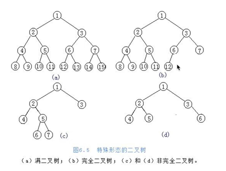
Storage method of binary tree (representation method)
- Chain storage method
- Sequential storage method
Sequential storage method
- list
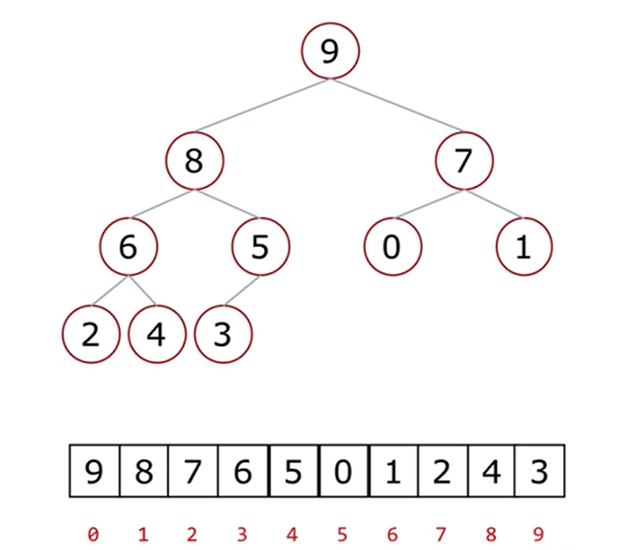
Number subscript relationship between parent node and left child node:
I = = > 2I + 1 from parent node = = > left child node
Number subscript relationship between parent node and right child node:
I = = > 2I + 2 from parent node = = > right child node
Subscript relationship between child node and parent node number:
I = = > (i-1) / / 2 from child node = = > parent node
Heap: a special complete binary tree structure
- Large root heap: a complete binary tree, satisfying that any node is larger than its child node
- Small root heap: a complete binary tree, satisfying that any node is smaller than its child node
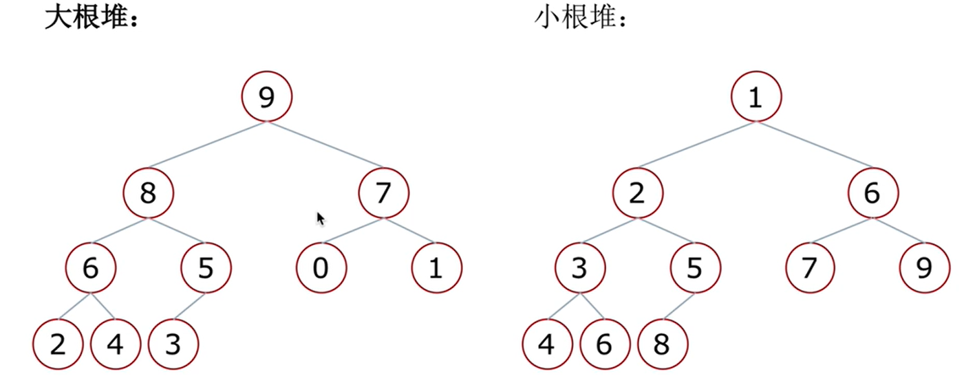
Downward adjustment of heap
- Suppose that the left and right subtrees of the root node are heaps, but the root node is dissatisfied with the nature of heaps
- When the left and right subtrees of the root node are heaps, they can be transformed into a heap through a downward adjustment
Heap sorting process
- Build a heap (adjust down from the last non leaf node to the last non leaf node)
- Get the top element, which is the largest element
- Remove the top of the heap and put the last element of the heap on the top of the heap
- The top element is the second largest element
- Repeat step 3 until the reactor becomes empty
Principle: when sorting from small to large, the large top heap is used. Each time, the top elements of the heap are taken and exchanged with the following elements, and then the remaining elements are sorted by the large top heap.
Heap sorting: topk problem
- Now there are n numbers. Design the algorithm to get the number with the largest K. (k<n)
- Solution:
- Slice after sorting( O ( n l o g n ) O(nlogn) O(nlogn)+k) can be rounded off K
- Bubble, insert, select, sort( O ( k n ) O(kn) O(kn))
- Heap sorting idea,
O
(
n
l
o
g
k
)
O(nlogk)
O(nlogk)
- Take the first k elements of the list to create a small root heap. The top of the heap is the K largest number at present
- Traverse the original list backward in turn. If the element in the list is smaller than the top of the heap, the element will be ignored; If it is larger than the heap top, the heap top is replaced with this element, and the heap is adjusted successively;
- After traversing all the elements in the list, pop up the top of the heap in reverse order

# Heap sorting - the most difficult

def sift(lis, low, high):
    '''

    :param lis: list
    :param low: Root node location of heap
    :param high: Position of the last element of the heap
    :return:
    '''

    i = low # i first points to the root node, and the whole process refers to the parent class
    j = 2*i + 1 # Left child
    tmp = lis[i] # Store the top of the pile
    while j <= high:
        if j+1 <= high and lis[j+1] > lis[j]: # If the right child has and is older
            j = j + 1 # j points to the right child
        if lis[j] > tmp:
            lis[i] = lis[j]
            i = j               # Look down one floor
            j = 2*i + 1
        else:               # tmp is bigger. Put tmp in a leading position
            break
    lis[i] = tmp            # Put tmp on leaf node

def heap_sort(lis):
    n = len(lis)
    for i in range((n-2)//2, -1, -1):
        # i indicates the subscript of the root of the part adjusted during heap building:
        sift(lis, i, n-1)
    # Reactor building is complete
    for i in range(n-1, -1, -1):
        # i points to the last element of the current heap
        lis[0] ,lis[i] = lis[i], lis[0]
        sift(lis, 0, i - 1) # i-1 is the new high

lis = list(range(100))
import random
random.shuffle(lis)

heap_sort(lis)
print(lis)
heap_sort(lis)
Built in module
# ---------------------------------System built-in heap sorting-----------------------------------
import heapq # Queue priority queue
import random
li = list(range(100))
random.shuffle(li)
print(li)
heapq.heapify(li) # Build pile
print(li)

n = len(li)
for i in range(n):
    print(heapq.heappop(li), end=',')
Problem: now there are n numbers. Design the algorithm to get the number with the largest K. (k<n)
Solution:
- Slice after sorting( O ( n l o g n ) O(nlogn) O(nlogn)+k) can be rounded off K
- Bubble, insert, select, sort( O ( k n ) O(kn) O(kn))
- Heap sorting idea,
O
(
n
l
o
g
k
)
O(nlogk)
O(nlogk)
- Take the first k elements of the list to create a small root heap. The top of the heap is the K largest number at present
- Traverse the original list backward in turn. If the element in the list is smaller than the top of the heap, the element will be ignored; If it is larger than the heap top, the heap top is replaced with this element, and the heap is adjusted successively;
- After traversing all the elements in the list, pop up the top of the heap in reverse order
code implementation
# Small root pile
def sift(lis, low, high):
    '''

    :param lis: list
    :param low: Root node location of heap
    :param high: Position of the last element of the heap
    :return:
    '''

    i = low # i first points to the root node, and the whole process refers to the parent class
    j = 2*i + 1 # Left child
    tmp = lis[i] # Store the top of the pile
    while j <= high:
        if j+1 <= high and lis[j+1] < lis[j]: # If the right child has and is older
            j = j + 1 # j points to the right child
        if lis[j] < tmp:
            lis[i] = lis[j]
            i = j               # Look down one floor
            j = 2*i + 1
        else:               # tmp is bigger. Put tmp in a leading position
            break
    lis[i] = tmp            # Put tmp on leaf node

def topk(li, k):
    heap = li[0:k]
    for i in range((k-2)//2, -1, -1):
        sift(heap, i, k-1)
    # 1. Pile building
    for i in range(k, len(li)-1):
        if li[i] > heap[0]:
            heap[0] = li[i]
            sift(heap, 0, k-1)
    # 2. Traversal
    for i in range(k - 1, -1, -1):
        heap[0], heap[i] = heap[i], heap[0]
        sift(heap, 0, i - 1)
    # 3. Counting
    return heap

import random
li = list(range(1000))
random.shuffle(li)
print(topk(li,10))
6. Merge and sort (additional space)
Merge sort is to divide the sequence to be sorted into several subsequences, and each subsequence is orderly. Then the ordered subsequences are combined into an overall ordered sequence.

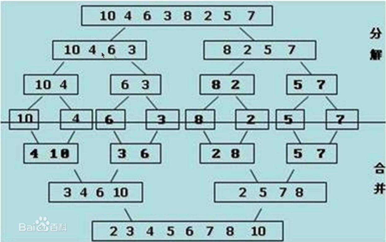
Summary: quick sort, heap sort and merge sort
The time complexity of the three sorting algorithms is O ( n l o g n ) O(nlogn) O(nlogn)
In general, in terms of running time:
- Quick sort < merge sort < heap sort
Disadvantages of three sorting algorithms:
- Quick sort: in extreme cases, the sorting efficiency is low
- Merge sort: requires additional memory overhead
- Heap sorting: relatively slow in fast sorting algorithms
7. Hill sort
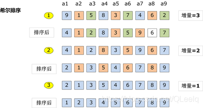
Principle: Hill sort is an improved algorithm of insertion sort. It is an efficient implementation of insertion sort, also known as reduced incremental sort. Hill's sorting step size is adjusted from large to small, so the step size is the key. The final step size is 1 to make the final sorting.
When the step size is 1, the matching sequence can be discharged.
Hill sort is a variant of insertion sort. Hill sort is a grouping insertion sort algorithm
The implementation steps are as follows:
- First take an integer d 1 = n / 2 d_1=n/2 d1 = n/2, dividing the element into d 1 d_1 d1) groups, the distance between adjacent quantity elements of each group is d 1 d_1 d1, direct insertion sorting in each group
- Take the second integer d 2 = d 1 / 2 d_2=d_1/2 d2 = d1 / 2, repeat the above grouping sorting process until d i = 1 d_i=1 di = 1, that is, all elements are directly inserted and sorted in the same group
- Hill sorting does not make some elements orderly, but makes the overall data more and more orderly; The last sorting makes all the data orderly
Hill sort is slower than heap sort (NB trio)
The choice of gap is different, and the time complexity is different (there are still big guys studying it at present)
The Python code is implemented as follows:
def insert_sort_gap(lis, gap): # Change the 1 inserted in the sort to gap
    for i in range(len(lis)):
        temp = lis[i]
        j = i - gap
        while j >= 0 and lis[j] > temp:
            lis[j+gap] = lis[j]
            j -= gap
        lis[j+gap] = temp

def shell_sort(lis):
    d = len(lis) // 2
    while d >= 1:
        insert_sort_gap(lis, d)
        d //= 2

lis = [3,1,2,4,5,7,6]
shell_sort(lis)
print(lis)
8. Counting and sorting (extra space)
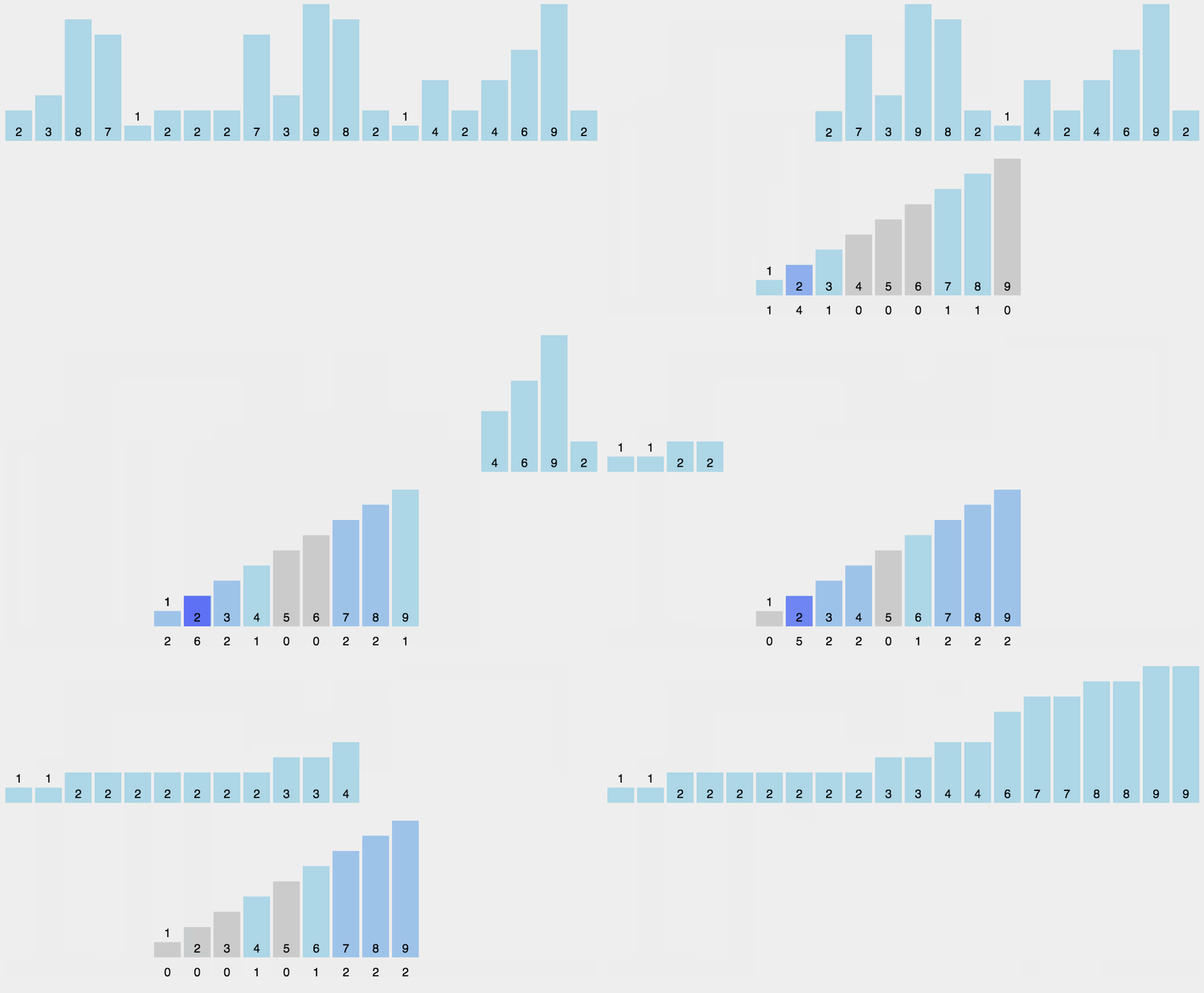
Principle: when the value of the number to be sorted is an integer within a certain range, you can use the number to be sorted as the subscript of the counting array, count the number of each number, and then output it in turn.
Algorithm steps:
- Take O(n) to scan the whole sequence A and find the maximum value of the sequence: max
- Open up a new space and create a new array B with a length of (max + 1)
- The value recorded by the index element in array B is the number of times an element in A appears
- Finally, the target integer sequence is output. The specific logic is to traverse array B and output the corresponding elements and the corresponding number
Sort the list. It is known that the number in the list ranges from 0 to 100. The design time complexity is O ( n ) O(n) O(n) algorithm
It is fast and faster than the sorting of the system, but it has many limitations. For example, it needs to use additional memory space, the maximum number is not necessarily clear, and there are problems such as decimals that cannot be solved
9. Bucket sorting (additional space)
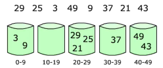
Bucket sorting transformation counting sorting
Bucket sorting: first, divide the elements into different buckets and sort the elements in each bucket.
The performance of bucket sorting depends on the distribution of data, that is, different bucket sorting strategies need to be adopted for different data sorting
def bucket_sort(lis, n=100, max_num=10000):
    buckets = [[] for _ in range(n)] # Create bucket
    for var in lis:
        i = min(var // (max_num // n), n-1) # i indicates the number of buckets var is put in
        buckets[i].append(var) # Add var to the bucket
        # Keep the order in the bucket and sort
        for j in range(len(buckets[i])-1, 0, -1):
            if buckets[i][j-1] > buckets[i][j]:
                buckets[i][j-1], buckets[i][j] = buckets[i][j], buckets[i][j-1]
            else:
                break

    sorted_lis = []
    for buc in buckets:
        sorted_lis.extend(buc)
    return sorted_lis

import random
lis = [random.randint(0,10000) for _ in range(1000)]
print(bucket_sort(lis))
10. Cardinality sorting
Multi keyword sorting: there is now an employee table, which requires sorting by salary, and employees of the same age are sorted by age.
- Sort by age first, and then sort stably by salary
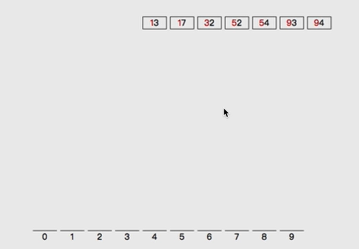
Can the sorting of 32, 13, 94, 52, 17, 54 and 91 be regarded as multi keyword sorting
Sort the following numbers by multiple keywords:
- Carry out similar bucket sorting operation with the size of single digit number
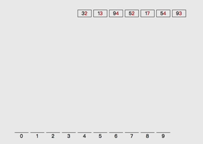
- The results of barrel separation are as follows:

- Sort by bucket:
- It can ensure that the number is directly calculated according to the sorting result when sorting by ten digits
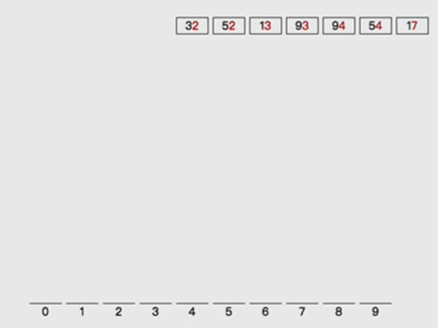
- Divide barrels according to ten digits

- Put the numbers out of the bucket one by one
def radix_sort(li):
    max_num = max(li) # Maximum
    it = 0
    while 10 ** it <= max_num:
        buckets = [[] for _ in range(10)] # Create 10 buckets
        for val in li:
            digit = (val // 10% of it now * * #
            buckets[digit].append(val)
        # Completion of barrel separation
        li.clear()
        for buc in buckets:
            li.extend(buc)
        # Rewrite the number back to li
        it += 1

import random
li = list(range(1000))
random.shuffle(li)
radix_sort(li)
print(li)