Initial value of weight

(the pit here is too deep. This article is just an introduction to in-depth learning and will not pursue theory in detail)

In the learning of neural network, the initial value of weight is particularly important. In fact, what kind of weight initial value is set is often related to the success of neural network learning. This section will introduce the recommended value of the initial value of weight, and confirm whether the learning of neural network will be carried out quickly through experiments.

2.1 asymmetric structure

In the error back propagation method, all weight values will be updated the same. For example, in a two-layer neural network, assume that the weights of layer 1 and layer 2 are 0. In this way, when propagating forward, because the weight of the input layer is 0, all neurons in layer 2 will be passed the same value. All neurons in layer 2 input the same value, which means that the weights of layer 2 will be updated the same during back propagation (recall "back propagation of multiplication nodes"). Therefore, the weights are updated to the same value and have symmetrical values (duplicate values). This makes neural networks lose many different weights. In order to prevent "weight homogenization" (strictly speaking, to disintegrate the symmetrical structure of weight), the initial value must be randomly generated.

2.2 distribution of activation values of hidden layers

Observing the distribution of the activation value A (the output data of the activation function) of the hidden layer can get A lot of inspiration. Here, let's do A simple experiment to observe how the initial value of weight affects the distribution of activation value of hidden layer. The experiment to be done here is to input randomly generated input data to A five layer neural network (the activation function uses sigmoid function), and draw the data distribution of activation values of each layer with histogram. This experiment refers to the course CS231n of Stanford University. This is A very good course for computer vision and in-depth learning.

import numpy as np
import matplotlib.pyplot as plt

def sigmoid(x):
    return 1/(1+np.exp(-x))

x = np.random.randn(1000,100)
node_num = 100 #Number of nodes in each hidden layer
hidden_layer_size = 5 #5 hidden layers
activations = {} #Dictionary for saving active values
no_activations={}
for i in range(hidden_layer_size):
    if i != 0:
        x = activations[i-1]

    w = np.random.randn(node_num,node_num)*1

    z = np.dot(x,w)
    a = sigmoid(z)
    activations[i] = a
    no_activations[i] = z

for i,a in activations.items():
    plt.subplot(1,len(activations),i+1)
    plt.title(str(i+1)+"-layer")
    plt.hist(a.flatten(),30,range = (0,1))


print(activations[0].flatten().shape)
plt.show()

The number of hist statistics is 0 ~ 1 in the code. It is divided into 30 copies. How many data are there in each copy. Let's take a look

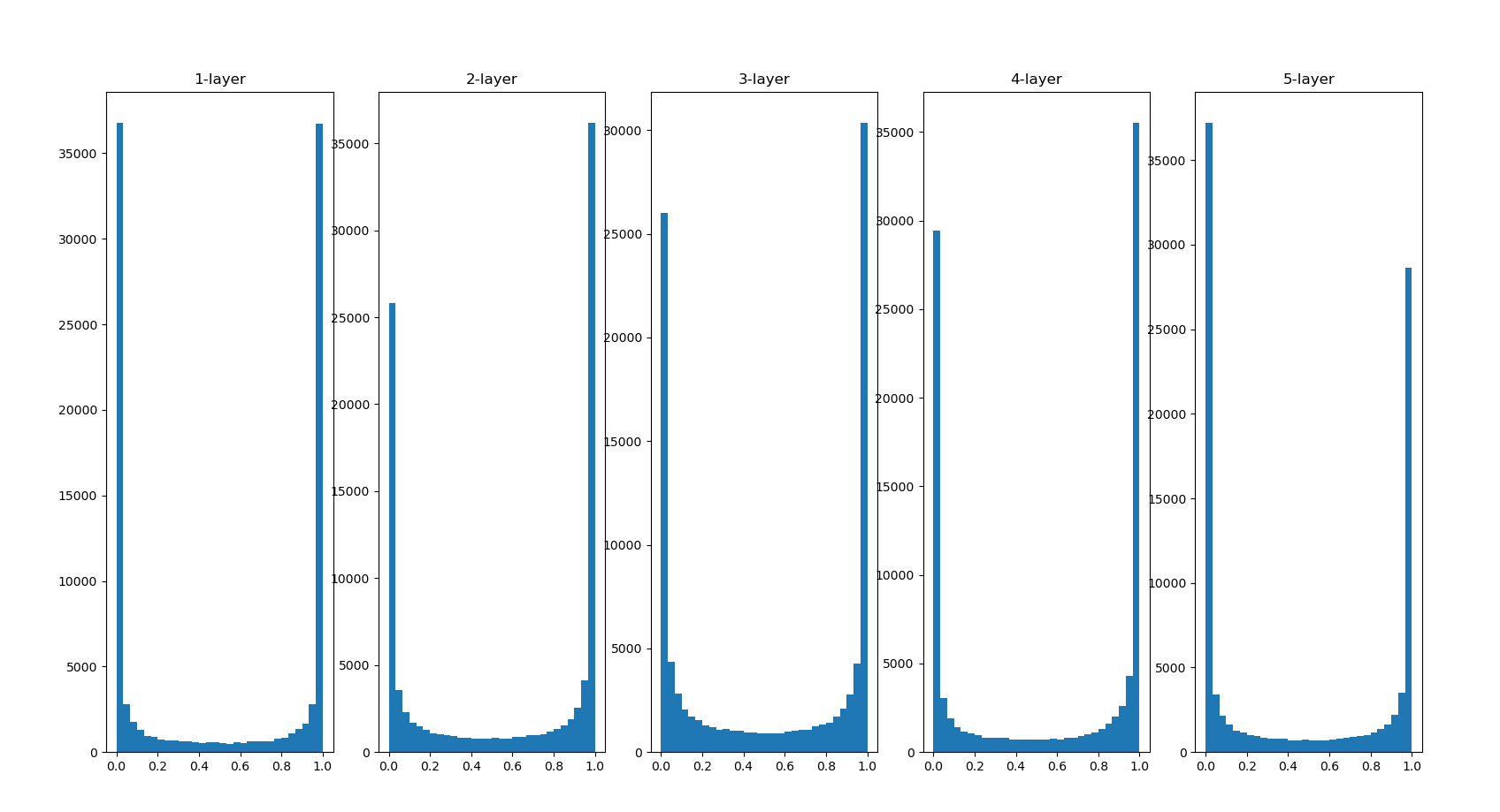
The activation values of each layer are biased towards 0 and 1. The sigmoid function used here is an S-type function. As the output keeps approaching 0 (or 1), the value of its derivative gradually approaches 0. Therefore, the data distribution biased towards 0 and 1 will cause the value of gradient in back propagation to become smaller and disappear at last. This problem is called gradient vanishing. In deep learning with deeper levels, the problem of gradient disappearance may be more serious.

Next, we transpose the weight to 0.01

import numpy as np
import matplotlib.pyplot as plt

def sigmoid(x):
    return 1/(1+np.exp(-x))

x = np.random.randn(1000,100)
node_num = 100 #Number of nodes in each hidden layer
hidden_layer_size = 5 #5 hidden layers
activations = {} #Dictionary for saving active values
no_activations={}
for i in range(hidden_layer_size):
    if i != 0:
        x = activations[i-1]

    w = np.random.randn(node_num,node_num)*0.01

    z = np.dot(x,w)
    a = sigmoid(z)
    activations[i] = a
    no_activations[i] = z
    
for i,a in activations.items():
    plt.subplot(1,len(activations),i+1)
    plt.title(str(i+1)+"-layer")
    plt.hist(a.flatten(),30,range = (0,1))

print(activations[0].flatten().shape)

plt.show()

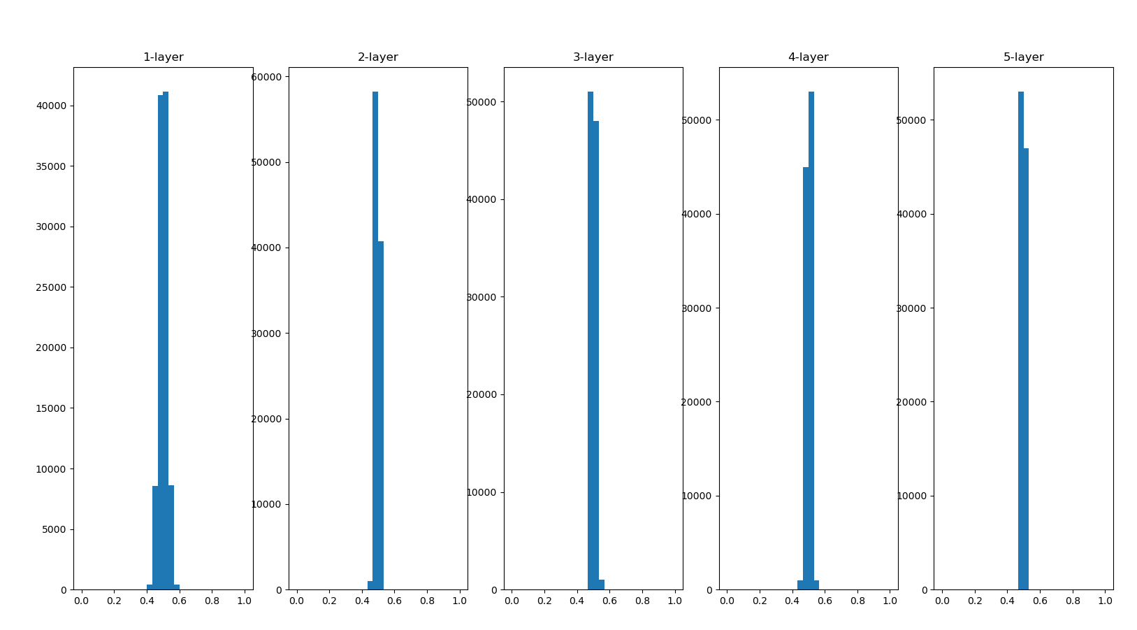
The distribution is concentrated around 0.5 this time. Because it is not biased towards 0 and 1 as in the previous example, the problem of gradient disappearance will not occur. However, the distribution of activation values is biased, indicating that there will be great problems in expressiveness. Why do you say that? Because if multiple neurons output almost the same value, they have no meaning of existence. For example, if 100 neurons output almost the same value, one neuron can also express basically the same thing. Therefore, the activation value is biased in the distribution, which will lead to the problem of "limited expressiveness".

The distribution of activation values of each layer requires an appropriate breadth. Why? Because by transferring diverse data between layers, neural networks can learn efficiently. Conversely, if biased data is transmitted, the gradient will disappear or the problem of "limited expressiveness" will appear, resulting in the failure of learning.

In Xavier's paper, in order to make the activation values of each layer show the same wide distribution, an appropriate weight scale is derived. The conclusion is that if the number of nodes in the previous layer is n, the standard deviation of the initial value is 1 / root n.

import numpy as np
import matplotlib.pyplot as plt

def sigmoid(x):
    return 1/(1+np.exp(-x))

x = np.random.randn(1000,100)
node_num = 100 #Number of nodes in each hidden layer
hidden_layer_size = 5 #5 hidden layers
activations = {} #Dictionary for saving active values
no_activations={}
for i in range(hidden_layer_size):
    if i != 0:
        x = activations[i-1]

    w = np.random.randn(node_num,node_num)*1/np.sqrt(node_num)

    z = np.dot(x,w)
    a = sigmoid(z)
    activations[i] = a
    no_activations[i] = z
    
for i,a in activations.items():
    plt.subplot(1,len(activations),i+1)
    plt.title(str(i+1)+"-layer")
    plt.hist(a.flatten(),30,range = (0,1))

print(activations[0].flatten().shape)

plt.show()

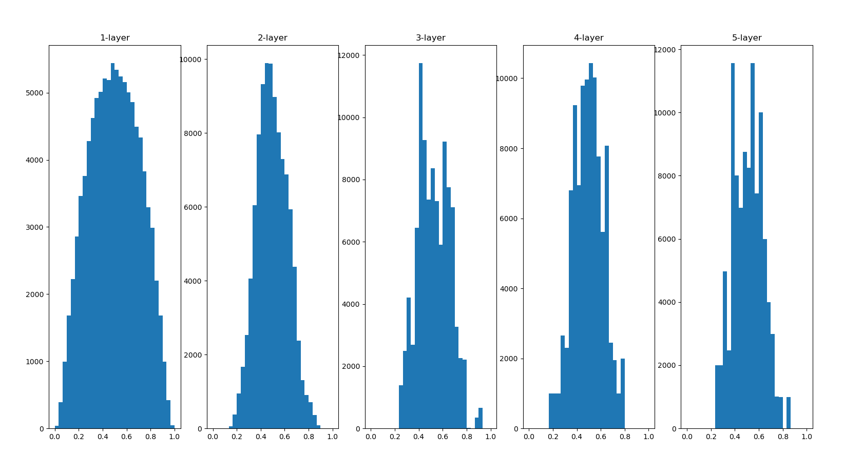
It can be seen from this result that the more the back layer, the more skewed the image becomes, but it presents a wider distribution than before. Because the breadth of moid is not limited by the appropriate performance of sigid, it is expected to transfer data between layers

The distribution of the back layer is slightly skewed. If we use tanh function (hyperbolic function) instead of sigmoid function, this slightly skewed problem can be improved. In fact, using the tanh function, it will have a beautiful bell shaped distribution. Both tanh function and sigmoid function are S-shaped curve functions, but tanh function is an S-shaped curve symmetrical about the origin (0,0), while sigmoid function is an S-shaped curve symmetrical about (x, y) = (0,0.5). It is well known that the function used as the activation function should preferably have the property of symmetry about the origin.

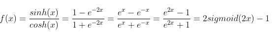
tanh function:

import numpy as np
import matplotlib.pyplot as plt

def sigmoid(x):
    return 1/(1+np.exp(-x))
def tanh(x):
    return 2*sigmoid(2*x)-1
x = np.random.randn(1000,100)
node_num = 100 #Number of nodes in each hidden layer
hidden_layer_size = 5 #5 hidden layers
activations = {} #Dictionary for saving active values
no_activations={}
for i in range(hidden_layer_size):
    if i != 0:
        x = activations[i-1]
        
    w = np.random.randn(node_num,node_num)*1/np.sqrt(node_num)

    z = np.dot(x,w)
    #a = sigmoid(z)
    a = tanh(z)
    activations[i] = a
    no_activations[i] = z

for i,a in activations.items():
    plt.subplot(1,len(activations),i+1)
    plt.title(str(i+1)+"-layer")
    plt.hist(a.flatten(),30,range = (0,1))

print(activations[0].flatten().shape)
plt.show()

Indeed, I don't see anything like a bell.

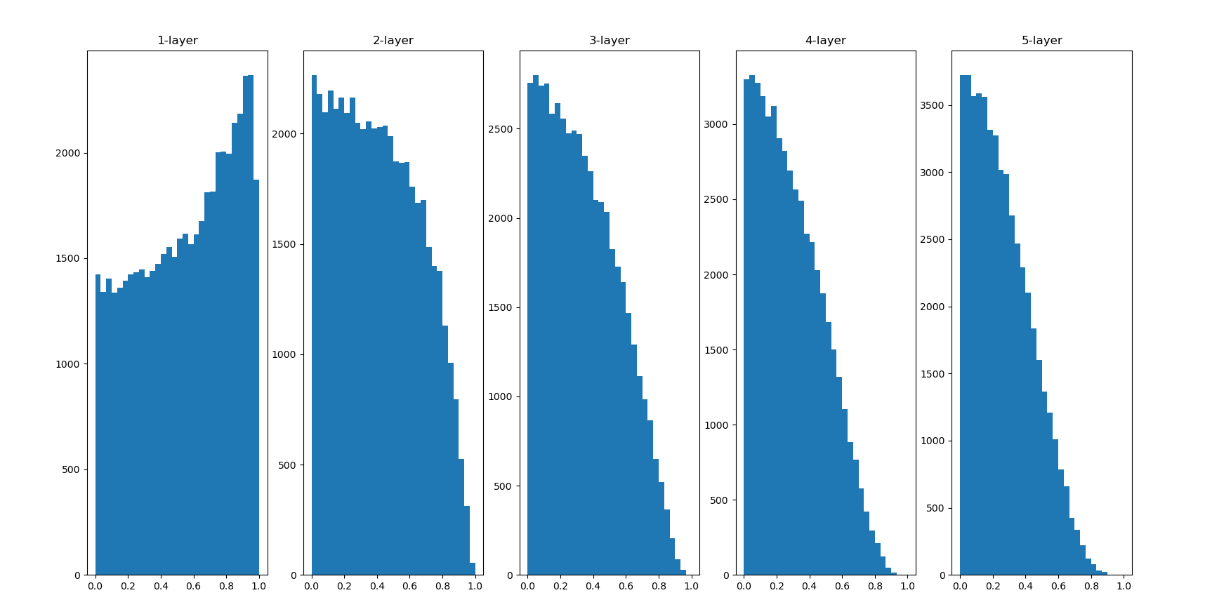
Xavier initial value is derived on the premise that the activation function is a linear function. Because sigmoid function and tanh function are symmetrical left and right, and the vicinity of the center can be regarded as a linear function, it is suitable to use Xavier initial value. However, when the activation function uses ReLU, it is generally recommended to use the initial value dedicated to ReLU, that is, the initial value recommended by Kaiming He et al., also known as "He initial value". The initial value is under the root sign (2/n).

Let's try:

import numpy as np
import matplotlib.pyplot as plt

def ReLU(x):
    temp = x<=0
    x[temp] = 0
    return x

node_num = 100 #Number of nodes in each hidden layer
hidden_layer_size = 5 #5 hidden layers
activations = {} #Dictionary for saving active values
active_init = {"The initial value of the weight is 0, and the standard deviation is 0.01 Gaussian distribution of":0.01,
               "The initial weight value is Xavier Initial value":1/np.sqrt(node_num),
               "The initial weight value is He Initial value":np.sqrt(2 / node_num)}

for key,val in active_init.items():
    x = np.random.randn(1000, 100)
    for i in range(hidden_layer_size):
        if i != 0:
            x = activations[i - 1]

        w = np.random.randn(node_num, node_num) * val
        print(val)
        z = np.dot(x, w)
        a = ReLU(z)
        activations[i] = a

    plt.figure(key)
    plt.xlabel(key)

    for i, a in activations.items():
        plt.subplot(1, len(activations), i + 1)
        plt.title(str(i + 1) + "-layer")
        plt.hist(a.flatten(), 30, range=(0, 1))

    activations = {}


plt.show()

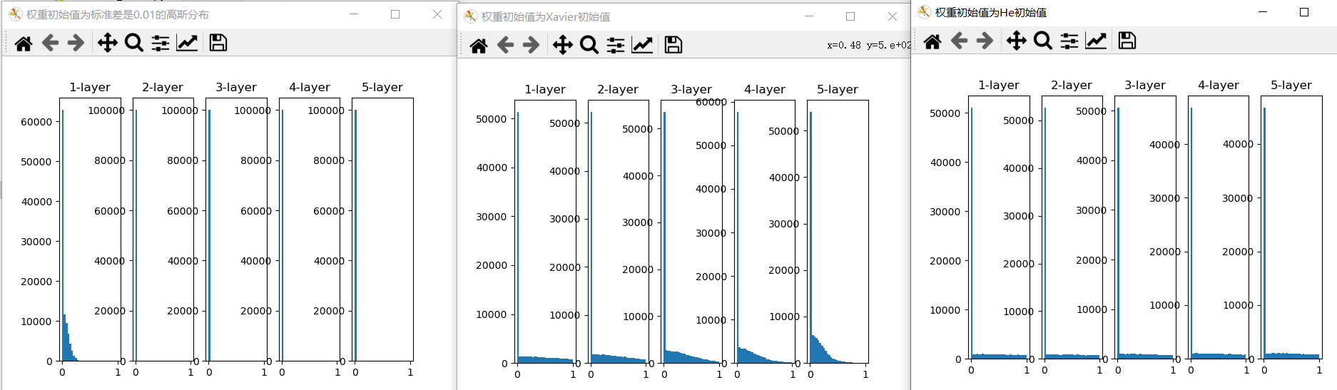
According to the experimental results, when "std = 0.01", the activation value of each layer is very small A. The value transmitted on the neural network is very small, which indicates that the gradient of weight in reverse propagation is also very small. This is A very serious problem. In fact, there is basically no progress in learning.

Next is the result when the initial value is Xavier initial value. In this case, as the layer deepens, the bias becomes larger. In fact, when the layer deepens, the bias of activation value becomes larger, and the gradient disappears during learning. When the initial value is He initial value, the distribution width in each layer is the same. Since the breadth of data can remain unchanged even if the layer is deepened, appropriate values will be passed during reverse propagation. To sum up, when the activation function uses ReLU, the initial value of weight uses He initial value, and when the activation function is sigmoid or tanh S-curve function, the initial value uses Xavier initial value. This is current best practice

In the previous chapters, we identified the mnist data set. Now we do an experiment with the mnist data set again to observe to what extent the assignment methods of different initial values of weights will affect the learning of neural network. The book uses a five layer fully connected neural network. We have made a three-layer one in the chapter of error back propagation before. Try the three-layer one. The previous code is here Error back propagation code . We are interested in bp_two_layer_net.py and train_bp_two_neuralnet.py has been transformed. If you don't want to download, you can see the notes in this chapter, including the code mnist data set recognition based on error back propagation.

The appearance after transformation is as follows

Firstly, the three-layer neural network is changed, which changes the initialization parameters from the original weight_ init_ Change STD to weight_init_std1,weight_init_std2，bp.net_layer comes from the error back propagation code. It is the implementation of various layers, numerical_gradient is the derivative of differential method. It is not used in this example. Just ignore it.

import numpy as np
from collections import OrderedDict
from bp.net_layer import *
from deeplearning.fuction import numerical_gradient

class TwoLayerNet:
    def __init__(self,input_size,hidden_size,output_size,
                 weight_init_std1,weight_init_std2):
        #Initialize weight
        self.params = {}
        self.params['W1'] = weight_init_std1*np.random.randn(input_size,hidden_size)
        self.params['b1'] = np.zeros(hidden_size)
        self.params['W2'] = weight_init_std2*np.random.randn(hidden_size,output_size)
        self.params['b2'] = np.zeros(output_size)

        """
        OrderedDict It's an ordered dictionary
        """
        #Generation layer
        self.layers = OrderedDict()
        self.layers['Affine1'] = Affine(self.params['W1'],self.params['b1'])
        self.layers['Relu1'] = Relu()
        self.layers['Affine2'] = Affine(self.params['W2'],self.params['b2'])

        self.lastLayer = SoftMaxTithLoss()

    #The function of ordered dictionary is to spread forward
    def predict(self,x):
        for layer in self.layers.values():
            x = layer.forward(x)

        return x

    #The loss function y we obtained before is after softmax, but the current predict does not go through softmax
    def loss(self,x,t):
        y = self.predict(x)

        return self.lastLayer.forward(y,t)

    def accuracy(self,x,t):
        y = self.predict(x)         #y score
        y = np.argmax(y,axis = 1)   #Get the highest score without softmax y
        if t.ndim != 1 :            #If t is 1D, axis=1 will make an error, mini_batch won't be 1D
            t = np.argmax(t,axis = 1)
        acuracy = np.sum((y==t)/float(x.shape[0]))

        return acuracy

    #Numerical differentiation for gradient
    def numerical_gradient(self,x,t):
        loss_W = lambda W:self.loss(x,t)

        grads = {}
        grads['W1'] = numerical_gradient(loss_W,self.params['W1'])
        grads['b1'] = numerical_gradient(loss_W, self.params['b1'])
        grads['W2'] = numerical_gradient(loss_W, self.params['W2'])
        grads['b2'] = numerical_gradient(loss_W, self.params['b2'])

        return grads

    #Error back propagation gradient
    def gradient(self,x,t):
        #forward propagation is the process of obtaining the value of the loss function
        self.loss(x,t)

        #backward
        dout = 1
        dout = self.lastLayer.backward(dout)

        layers = list(self.layers.values())
        layers.reverse()

        for layer in layers:
            dout = layer.backward(dout)

        grads = {}
        grads['W1'] = self.layers['Affine1'].dW
        grads['b1'] = self.layers['Affine1'].db
        grads['W2'] = self.layers['Affine2'].dW
        grads['b2'] = self.layers['Affine2'].db

        return grads

Then we began to train three networks and put the pictures on them. I wrote a lot of notes. I believe it will be easy to understand if you read the chapter of error back propagation or understand error back propagation.

from bp_two_layer_net_adaptive import TwoLayerNet
import numpy as np
from deeplearning.mnist import load_mnist
import matplotlib.pyplot as plt


(x_train,t_train),(x_test,t_test) = load_mnist(normalize=True,one_hot_label=True)

# Three neural networks with different initial weights
network_std = TwoLayerNet(input_size=784,hidden_size=50,output_size=10,
                          weight_init_std1=0.01,weight_init_std2=0.01)
network_Xavier = TwoLayerNet(input_size=784,hidden_size=50,output_size=10,
                             weight_init_std1=1/np.sqrt(784),weight_init_std2=1/np.sqrt(50))
network_He = TwoLayerNet(input_size=784,hidden_size=50,output_size=10,
                         weight_init_std1=np.sqrt(2/784),weight_init_std2=np.sqrt(2/50))

my_network = {"std=0.01":network_std,"Xavier":network_Xavier,"He":network_He}




# We need three to record the value of the loss function. After all, there are three networks
train_loss_list_std = []
train_loss_list_Xavier = []
train_loss_list_He = []

my_train_loss_list = {"std=0.01":train_loss_list_std,"Xavier":train_loss_list_Xavier,"He":train_loss_list_He}

#We can't use these two. Let's draw a loss function diagram
#train_acc_list = []
#test_acc_list = []

#We don't need to calculate the correct rate
#iter_per_epoch = max(train_size/batch_size,1)

#Pay attention to recycle net_ The key is because there is a key for circulation. It can't be the same
for net_key,network in my_network.items():

    iters_num = 2000
    #Change here to 2000
    train_size = x_train.shape[0]
    batch_size = 100
    learning_rate = 0.1

    for i in range(iters_num):
        batch_mask = np.random.choice(train_size, batch_size)
        x_batch = x_train[batch_mask]
        t_batch = t_train[batch_mask]

        # Reverse error acquisition gradient
        grad = network.gradient(x_batch, t_batch)

        # Update gradient
        for key in ('W1', 'b1', 'W2', 'b2'):
            network.params[key] -= learning_rate * grad[key]

        loss = network.loss(x_batch, t_batch)
        #train_loss_list.append(loss)
        my_train_loss_list[net_key].append(loss)

    print("network"+net_key+"Training is over")

    """ We don't need to comment out the part of calculating the correct rate
        if i % iter_per_epoch == 0:
        train_acc = network.accuracy(x_train,t_train)
        test_acc = network.accuracy(x_test,t_test)
          train_acc_list.append(train_acc)
        test_acc_list.append(test_acc)

        print(train_acc,test_acc)"""

print("After three network training, start drawing:")
#Before drawing, let's modify the list of loss functions to make the results clear
#We take one data every 25 bits to avoid data overlap
for key in my_train_loss_list.keys():
    my_train_loss_list[key] = np.array(my_train_loss_list[key])
    b = np.arange(0, 2000, 25)
    my_train_loss_list[key]=my_train_loss_list[key][b]
    print(my_train_loss_list[key].shape)

#Draw a diagram with the list of the changes of the values of the three loss functions we get
plt.figure()


#Style of line
markers = {'std=0.01': 'o', 'Xavier': 's', 'He': 'D'}
#x is the same. It doesn't matter who you choose
x = np.arange(len(my_train_loss_list['Xavier']))
print(x)

for key,train_loss_list in my_train_loss_list.items():
    plt.plot(x,train_loss_list,label=key,marker=markers[key])





plt.xlabel("mini_batch*25")
plt.ylabel("loss")
plt.legend()

"""
The accuracy of test data and training data can't be used
f2 = plt.figure()
x2 = np.arange(len(train_acc_list))

y1 = np.array(train_acc_list)
y2 = np.array(test_acc_list)

plt.xlabel("mini_batch")
plt.ylabel("accuracy")
plt.plot(x2,y1,label="train data")
plt.plot(x2,y2,linestyle="--",label="test data")
plt.legend()
"""
plt.show()

Although we have dealt with the list of loss functions and took a value every 25 bits, it still doesn't seem easy to see. Let's start with "magic".

import numpy as np

def smooth_curve(x):
    """Piecewise smooth curve is used to make the graph of loss function smooth"""
    
    window_len = 11
    s = np.r_[x[window_len-1:0:-1], x, x[-1:-window_len:-1]]
    w = np.kaiser(window_len, 2)
    y = np.convolve(w/w.sum(), s, mode='valid')
    return y[5:len(y)-5]

Then slightly modify the training code and add only one smooth_curve function. As for the theory of piecewise smooth curve, we don't need to understand it for the time being. When we use it, we can copy it directly.

for key,train_loss_list in my_train_loss_list.items():
    plt.plot(x,smooth_curve(train_loss_list),label=key,marker=markers[key])

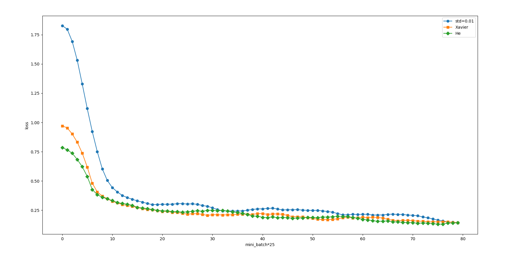
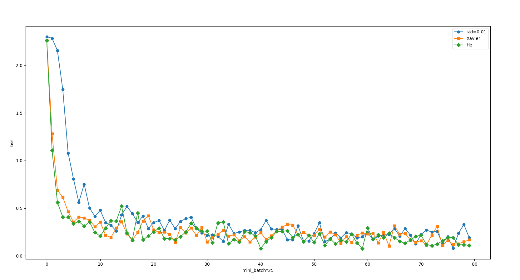
Our curve becomes much smoother. In fact, it is easy to see that the initial values of Xavier and he are much better than 0.01, and he seems to be a little better than Xavier. But don't forget that we have a three-layer neural network, input layer 784, hidden layer 50 and output layer 10. This neural network is too small. What if we replace it with a five layer neural network? The examples given in the book are shown in the figure below.

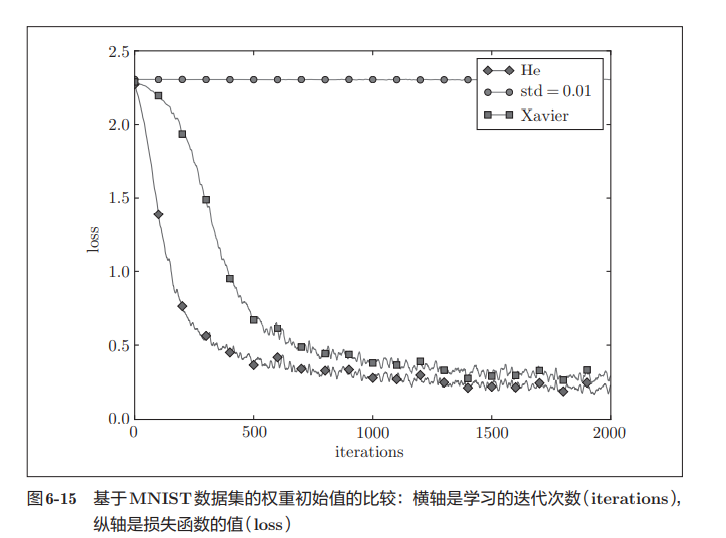
In this experiment, the neural network has five layers, each layer has 100 neurons, and the activation function uses ReLU. It can be seen from the results of the above figure that learning is completely impossible when std = 0.01. This is the same as the distribution of activation values just observed, because the value transmitted in the forward propagation is very small (data concentrated near 0). Therefore, the gradient obtained during reverse propagation is also very small, and the weight is hardly updated. On the contrary, when the weight initial value is Xavier initial value and He initial value, the learning goes well. Moreover, we find that the learning progress is faster when He is the initial value.