Extension end tecdat| [Video] CNN (convolutional neural network) model and R language implementation

Posted by bdemo2 on Tue, 15 Feb 2022 08:09:51 +0100

Original link: http://tecdat.cn/?p=18149

Original source: Tuo end data tribal official account

Driverless cars can be traced back to 1989. Neural networks have existed for a long time. What are the reasons for the upsurge of artificial intelligence and deep learning in recent years? [1 second] part of the answer lies in Moore's law and the significant improvement of hardware and computing power. We can get twice the result with half the effort now. As the name suggests, the concept of neural network is inspired by our own brain neural network. Neurons are very long cells. Each cell has a process called dendrite, which receives and transmits electrochemical signals from surrounding neurons. As a result, our brain cells form a flexible and powerful communication network. This distribution process similar to the assembly line supports complex cognitive abilities, such as music playing and painting.

https://www.bilibili.com/vide...

Video: CNN (convolutional neural network) model and R language implementation

Neural network structure

Neural networks usually contain an input layer, one or more hidden layers and an output layer. The input layer consists of p prediction variables or input units / nodes. Needless to say, it is usually best to standardize variables. These input units may be connected to one or more hidden units in the first hidden layer. A hidden layer that is completely connected to the previous layer is called a dense layer. In the figure, both hidden layers are dense.

Calculation and prediction of output layer

The output layer calculates the prediction, in which the number of units is determined by the specific problem. Generally, two classification problems need one output unit, while multi class problems with K categories will need K corresponding output units. The former can simply use the S-shaped function to directly calculate the probability, while the latter usually needs softmax transformation to add all the values in all k output units to 1, so it can be regarded as probability. No classification prediction is required.

weight

Each arrow shown in the figure passes the input associated with the weight. Each weight is essentially one of many coefficient estimates that help calculate the regression in the node pointed by the corresponding arrow. These are unknown parameters and must be adjusted by the model using the optimization process to minimize the loss function. Before training, all ownership weights are initialized with random values.

Optimization and loss function

Before training, we need to do two things well. One is the measurement of goodness of fit, which is used to compare the predictions and known labels of all training observations; The second is the optimization method of calculating gradient descent, which essentially adjusts all weight estimates at the same time to improve the direction of goodness of fit. For each method, we have a loss function and an optimizer. There are many types of loss functions, all for the purpose of quantifying prediction errors, such as using cross entropy. Popular stochastic optimization methods such as Adam.

Convolutional neural network

Convolutional neural network is a special type of neural network, which can be well used in image processing. The "convolution" in the name is attributed to the square squares of pixels in the image processed by the filter. As a result, the model can mathematically capture key visual cues. For example, the beak of a bird can highly distinguish birds among animals. In the example described below, the convolutional neural network may process the beak structure along a series of transformation chains involving convolution, pooling and flattening. Finally, it will see that the relevant neurons are activated. Ideally, the probability of predicting birds is the largest in the competitive class.

The image can be represented as a numerical matrix based on color intensity. Monochrome images are processed by 2D convolution layer, while color images need 3D convolution layer. We use the former.
The kernel (also known as filter) convolutes the square blocks of pixels into scalars in the subsequent convolution layer, and scans the image from top to bottom.
In the whole process, the kernel performs element by element multiplication, and sums all the products into a value, which is passed to the subsequent convolution layer.
The kernel moves one pixel at a time. This is the step size of the sliding window used by the kernel for convolution, which is adjusted step by step. Larger step size means finer and smaller convolution features.
Pooling is the sampling from the convolution layer, which can present the main characteristics in the lower dimension, so as to prevent excessive quasi merging and reduce the computational demand. The two main types of pooling are average pooling and maximum pooling. Providing a kernel and a step size, merging is equivalent to convolution, but the average or maximum value of each frame is taken.
Finally, the convolution layer is transformed into a flat neural network. It lays a foundation for practical prediction.

R language implementation

They are very useful when we use CNN (convolutional neural network) models to train multidimensional types of data (such as images). We can also implement CNN model for regression data analysis. We used Python for CNN model regression before. In this video, we implemented the same method in R.
We use one-dimensional convolution function to apply CNN model. We need Keras R interface to use Keras neural network API in R. If it is not available in the development environment, you need to install it first. This tutorial covers:

Prepare data
Defining and fitting models
Prediction and visualization results
source code

Let's start by loading the libraries needed for this tutorial.

library(keras)
library(caret)

prepare

Data in this tutorial, we use the Boston housing data set as target regression data. First, we will load the data set and divide it into training and test sets.

set.seed(123)
boston = MASS::Boston
indexes = createDataPartition(boston$medv, p = .85, list = F)

train = boston\[indexes,\]
test = boston\[-indexes,\]

Next, we separate the X-input and y-output parts of training data and test data, and convert them to matrix type. As you may know, "medv" is the Y data output of the Boston housing dataset, which is the last column. The remaining columns are x input data.
Check dimensions.

dim(xtrain)
\[1\] 432  13

dim(ytrain)
\[1\] 432   1

Next, we will redefine the shape of x input data by adding another dimension.

dim(xtrain)
\[1\] 432  13   1

dim(xtest)
\[1\] 74 13  1

Here, we can extract the input dimension of keras model.

print(in_dim)
\[1\] 13  1

Defining and fitting models

We define Keras model and add one-dimensional convolution layer. The input shape changes to the one defined above (13,1). We added the Flatten and Dense layers and compiled them using the "Adam" optimizer.

model %>% summary()
\_\_\_\_\_\_\_\_\_\_\_\_\_\_\_\_\_\_\_\_\_\_\_\_\_\_\_\_\_\_\_\_\_\_\_\_\_\_\_\_\_\_\_\_\_\_\_\_\_\_\_\_\_\_\_\_\_\_\_\_\_\_\_\_\_\_\_\_\_\_\_\_
Layer (type)                    Output Shape                  Param #    
========================================================================
conv1d_2 (Conv1D)               (None, 12, 64)                192        
\_\_\_\_\_\_\_\_\_\_\_\_\_\_\_\_\_\_\_\_\_\_\_\_\_\_\_\_\_\_\_\_\_\_\_\_\_\_\_\_\_\_\_\_\_\_\_\_\_\_\_\_\_\_\_\_\_\_\_\_\_\_\_\_\_\_\_\_\_\_\_\_
flatten_2 (Flatten)             (None, 768)                   0          
\_\_\_\_\_\_\_\_\_\_\_\_\_\_\_\_\_\_\_\_\_\_\_\_\_\_\_\_\_\_\_\_\_\_\_\_\_\_\_\_\_\_\_\_\_\_\_\_\_\_\_\_\_\_\_\_\_\_\_\_\_\_\_\_\_\_\_\_\_\_\_\_
dense_3 (Dense)                 (None, 32)                    24608      
\_\_\_\_\_\_\_\_\_\_\_\_\_\_\_\_\_\_\_\_\_\_\_\_\_\_\_\_\_\_\_\_\_\_\_\_\_\_\_\_\_\_\_\_\_\_\_\_\_\_\_\_\_\_\_\_\_\_\_\_\_\_\_\_\_\_\_\_\_\_\_\_
dense_4 (Dense)                 (None, 1)                     33         
========================================================================
Total params: 24,833
Trainable params: 24,833
Non-trainable params: 0
\_\_\_\_\_\_\_\_\_\_\_\_\_\_\_\_\_\_\_\_\_\_\_\_\_\_\_\_\_\_\_\_\_\_\_\_\_\_\_\_\_\_\_\_\_\_\_\_\_\_\_\_\_\_\_\_\_\_\_\_\_\_\_\_\_\_\_\_\_\_\_\_

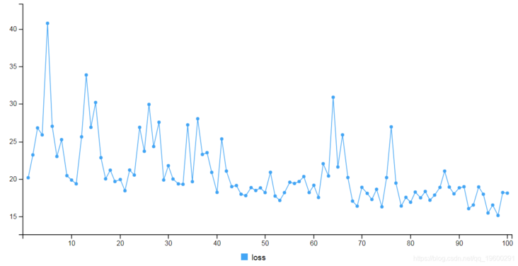
Next, we will use the training data to fit the model.

print(scores)
    loss 
24.20518

Prediction and visualization results

Now, we can use the trained model to predict the test data.

predict(xtest)

We will check the accuracy of the forecast through RMSE indicators.

cat("RMSE:", RMSE(ytest, ypred))
RMSE: 4.935908

Finally, we will visualize the results in the chart to check for errors.

x_axes = seq(1:length(ypred))

lines(x_axes, ypred, col = "red", type = "l", lwd = 2)
legend("topl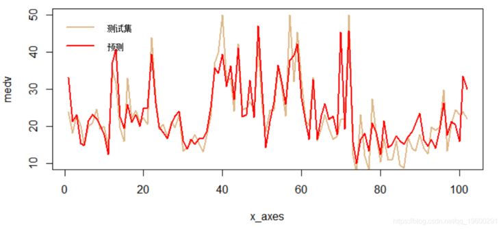

In this tutorial, we briefly learned how to use the keras CNN model in R to fit and predict regression data.

Programmer Think