1. General
1.1 industry background and pain points
Lithofacies analysis is a research work based on the microscopic description and classification of rock slices. It is also an important technology in the study of sedimentation and diagenesis. It has a basic guiding position for the engineering practice of oil and gas exploration and development. Through thin section analysis of mineral proportion, distribution, texture, pore space, cementation composition and other factors, it provides a better and more accurate means for the subsequent oil and gas field development scheme design as a guarantee. In engineering practice, most lithofacies analysis relies on a large number of geologists to use microscopes for visual inspection of rock slices. The contradiction between standards and time is becoming increasingly prominent. Generally speaking, there are three core pain points: first, human experts face a lot of heavy repetitive work, and the balance between energy and efficiency can not be ignored. At the same time, when many petrologists work together, there may be inconsistent analysis. Second, due to the differences in geological characteristics, development mechanism and other factors among oilfields distributed all over the world, cross source identification should be fully considered. Third, the existing automatic identification methods only target several types of specific blocks for the coverage of lithofacies; At the same time, it does not have the ability to migrate.
1.2 project value
In order to solve the above problems, we adopt a professional deep learning framework - flying paddle, which takes about 0.03 seconds to automatically identify a single sheet, and there is no lack of energy in the face of large-scale work area data. The cross source distribution of thin sections in different regions can also be optimized through the model based on large-scale training, and finally get a high-precision prediction model to accurately predict the distribution differences of different strata and different blocks. In view of the small coverage of the existing automation methods, we have adopted large-scale model training to cover more than 90% of the common lithofacies types and more than 95% of the scope required by the geological specialty. Uncovered lithofacies are not included in the analysis due to the scarcity of samples, but they can also be optimized by migration in the subsequent research process. The application of this method can not only complete the cross source large-scale hierarchical lithofacies analysis, but also accelerate and quantify various geological tasks and provide a basic migration basis.
2. Experimental process
2.1 data preparation and analysis
The data set of Nanjing University [1] includes more than 90% of the common rock types in the three types of rocks, and a total of 105 rock types are analyzed. The data set consists of 2634 pictures. The experiment randomly divides the data set into training set and test set in the proportion of 8:2.
# The code is subject to the warehouse
# Data loading
import paddle
import paddle.vision.transforms as T
def get_transforms():
    return T.Compose([
        T.Resize((224, 224)),
        T.ToTensor(),
        T.Normalize(mean=(0.485, 0.456, 0.406), std=(0.229, 0.224, 0.225))
    ])

def get_transforms_single():
    return T.Compose([
        T.Resize((224, 224)),
        T.ToTensor()
    ])


# Basic parameter configuration
train_parameters = {
    "data_dir": "data/data57425",  # Training data storage address
    "num_epochs": 10,
    "train_batch_size": 64,
    "infer_img": 'data/data57425/sunflowers/14646283472_50a3ae1395.jpg',


    "mean_rgb": [85, 96, 102],  # For the three channel mean value of commonly used pictures, it is usually necessary to make statistics on the training data first, and only the middle value is taken here

    "input_size": [3, 224, 224],
    "class_dim": -1,  # The number of categories will be obtained when initializing the custom reader
    "image_count": -1,  # The number of training pictures will be obtained when initializing the custom reader
    "label_dict": {},
    "train_file_list": "train.txt",
    "eval_file_list": "eval.txt",
    "label_file": "label_list.txt",
    "save_model_dir": "./save_dir/model",
    "continue_train": True,        # Whether to continue the last saved parameter training, with priority higher than the pre training model
    "image_enhance_strategy": {  # Image enhancement related strategies
        "need_distort": True,  # Enable image color enhancement
        "need_rotate": True,   # Need to add random angle
        "need_crop": True,      # Do you want to add clipping
        "need_flip": True,      # Do you want to add horizontal random flip
        "hue_prob": 0.5,  }
    }
2.2 data enhancement preprocessing module
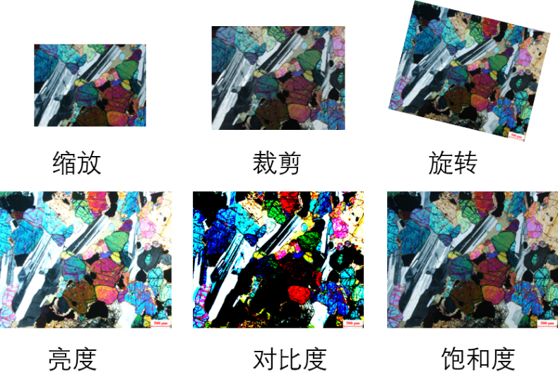
The storage space of a single sample of the original data set is about 1M. Compression under the condition of ensuring the image information can not only make the image lose the feature information, but also fully improve the number of samples that can be loaded in each batch and reduce the training cost of the model. Data enhancement technology is used to increase the robustness of the model. Figure 1 illustrates several ways of data enhancement: first, scale the picture to a specified size for the network to load; The random clipping strategy makes each part of the sample appear in the training process, and enhances the recognition ability of the model for the part of the picture; Enter in probability trigger mode
Row rotation, brightness, contrast and saturation are adjusted to simulate the experimental picture, which can be recognized in different cases.
2.3 network module design
In order to make full use of the inter channel characteristic information of the model in the network model, the mase resnext network structure adopts multi module nested design, as shown in Figure 2. 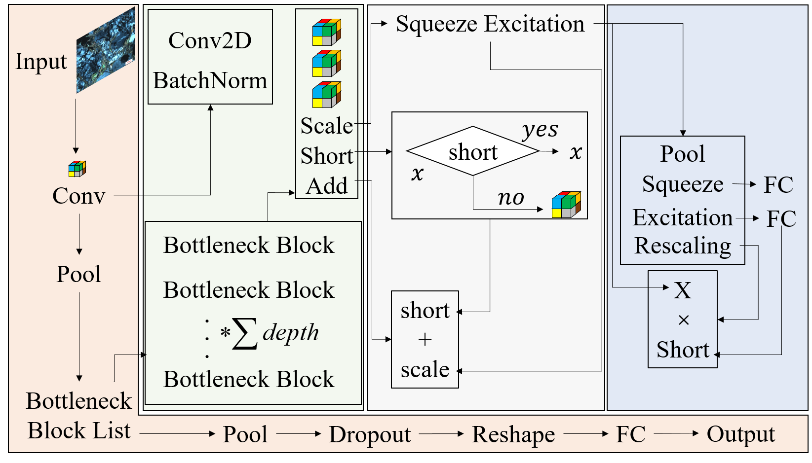
Mainline module: after inputting samples, it passes through Conv module to pool, stack the number of BottleneckBlock layers, pool, discard the probability, reorganize the characteristic shape, enter FC layer and output the type. Conv module: perform batch normalization after two-dimensional convolution calculation; BottleneckBlock: three times of Conv module stacking, SE module, Short module and Add module; SE module: pool layer, extrusion layer FC, excitation layer FC and Rescaling layer; Rescaling layer: perform matrix multiplication between the input value of SE module and the input value of Rescaling layer; Short module: judge whether the input attribute of the Short module adopts the Short strategy. If the answer is "yes", output the input value of the Short module. If the answer is "no", calculate and output the Conv module; Add module: matrix Add the output values of Short module and SE module, and take the result as the return value of BottleneckBlock module.
class BasicBlock(nn.Layer):
    expansion = 1

    def __init__(self,
                 inplanes,
                 planes,
                 stride=1,
                 downsample=None,
                 groups=1,
                 base_width=64,
                 dilation=1,
                 norm_layer=None):
        super(BasicBlock, self).__init__()
        # Determine whether it is a standard block
        if norm_layer is None:
            norm_layer = nn.BatchNorm2D

        if dilation > 1:
            raise NotImplementedError(
                "Dilation > 1 not supported in BasicBlock")
        # Define calculation operations
        self.conv1 = nn.Conv2D(
            inplanes, planes, 3, padding=1, stride=stride, bias_attr=False)
        self.bn1 = norm_layer(planes)
        self.relu = nn.ReLU()
        self.conv2 = nn.Conv2D(planes, planes, 3, padding=1, bias_attr=False)
        self.bn2 = norm_layer(planes)
        self.downsample = downsample
        self.stride = stride
    # Forward propagation
    def forward(self, x):
        identity = x

        out = self.conv1(x)
        out = self.bn1(out)
        out = self.relu(out)

        out = self.conv2(out)
        out = self.bn2(out)
        # Down sampling
        if self.downsample is not None:
            identity = self.downsample(x)

        out += identity
        out = self.relu(out)

        return out
# Define bottleneck block
class BottleneckBlock(nn.Layer):

    expansion = 4

    def __init__(self,
                 inplanes,
                 planes,
                 stride=1,
                 downsample=None,
                 groups=1,
                 base_width=64,
                 dilation=1,
                 norm_layer=None):
        super(BottleneckBlock, self).__init__()
        if norm_layer is None:
            norm_layer = nn.BatchNorm2D
        width = int(planes * (base_width / 64.)) * groups
        # Define calculation operations
        self.conv1 = nn.Conv2D(inplanes, width, 1, bias_attr=False)
        self.bn1 = norm_layer(width)

        self.conv2 = nn.Conv2D(
            width,
            width,
            3,
            padding=dilation,
            stride=stride,
            groups=groups,
            dilation=dilation,
            bias_attr=False)
        self.bn2 = norm_layer(width)

        self.conv3 = nn.Conv2D(
            width, planes * self.expansion, 1, bias_attr=False)
        self.bn3 = norm_layer(planes * self.expansion)
        self.relu = nn.ReLU()
        self.downsample = downsample
        self.stride = stride
    # Forward propagation

    def forward(self, x):
        identity = x

        out = self.conv1(x)
        out = self.bn1(out)
        out = self.relu(out)

        out = self.conv2(out)
        out = self.bn2(out)
        out = self.relu(out)

        out = self.conv3(out)
        out = self.bn3(out)
        # Judge whether to down sample

        if self.downsample is not None:
            identity = self.downsample(x)

        out += identity
        out = self.relu(out)

        return out

# Define mainline model

class MSRNet(nn.Layer):

    def __init__(self, block, depth, num_classes=751, with_pool=True,dropout_p = 0.4):
        super(MSRNet, self).__init__()
        layer_cfg = {
            18: [2, 2, 2, 2],
            34: [3, 4, 6, 3],
            50: [3, 4, 6, 3],
            101: [3, 4, 23, 3],
            152: [3, 8, 36, 3]
        }
        layers = layer_cfg[depth]
        self.num_classes = num_classes
        self.with_pool = with_pool
        self._norm_layer = nn.BatchNorm2D

        self.inplanes = 64
        self.dilation = 1

        self.conv1 = nn.Conv2D(
            3,
            self.inplanes,
            kernel_size=7,
            stride=2,
            padding=3,
            bias_attr=False)
        self.bn1 = self._norm_layer(self.inplanes)
        self.relu = nn.ReLU()
        self.maxpool = nn.MaxPool2D(kernel_size=3, stride=2, padding=1)
        self.layer1 = self._make_layer(block, 64, layers[0])
        self.layer2 = self._make_layer(block, 128, layers[1], stride=2)
        self.layer3 = self._make_layer(block, 256, layers[2], stride=2)
        self.layer4 = self._make_layer(block, 512, layers[3], stride=2)
        self.dropout = nn.Dropout(dropout_p) if dropout_p is not None else None
        self.batchnorm=nn.BatchNorm(2048)
        self.sigmoid = nn.Sigmoid()
        if with_pool:
            self.avgpool = nn.AdaptiveAvgPool2D((1, 1))

        if num_classes > 0:
            self.fc = nn.Linear(512 * block.expansion, num_classes)

    def _make_layer(self, block, planes, blocks, stride=1, dilate=False):
        norm_layer = self._norm_layer
        downsample = None
        previous_dilation = self.dilation
        if dilate:
            self.dilation *= stride
            stride = 1
        if stride != 1 or self.inplanes != planes * block.expansion:
            downsample = nn.Sequential(
                nn.Conv2D(
                    self.inplanes,
                    planes * block.expansion,
                    1,
                    stride=stride,
                    bias_attr=False),
                norm_layer(planes * block.expansion), )

        layers = []
        layers.append(
            block(self.inplanes, planes, stride, downsample, 1, 64,
                  previous_dilation, norm_layer))
        self.inplanes = planes * block.expansion
        for _ in range(1, blocks):
            layers.append(block(self.inplanes, planes, norm_layer=norm_layer))

        return nn.Sequential(*layers)


    def forward(self, x):
        x = self.conv1(x)
        x = self.bn1(x)
        x = self.relu(x)
        x = self.maxpool(x)
        x = self.layer1(x)
        x = self.layer2(x)
        x = self.layer3(x)
        x = self.layer4(x)

        if self.with_pool:
            x = self.avgpool(x)
        if self.dropout is not None:
            x = self.dropout(x)
        if self.num_classes > 0:
            x = paddle.flatten(x, 1)
            x1=self.batchnorm(x)
            x = self.fc(x1)
            #x= self.sigmoid(x)

        return x1,x
3, Experimental results and analysis
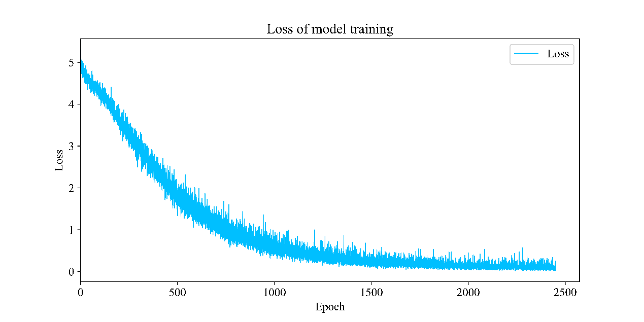
Figure 3 shows the loss function during model training, which tends to decrease with the increase of epoch. Although there is a loss in some training stages, there is no decline or even an upward trend, the model finally overcomes the trap of local optimization by deepening sample learning, so as to further reduce the loss.
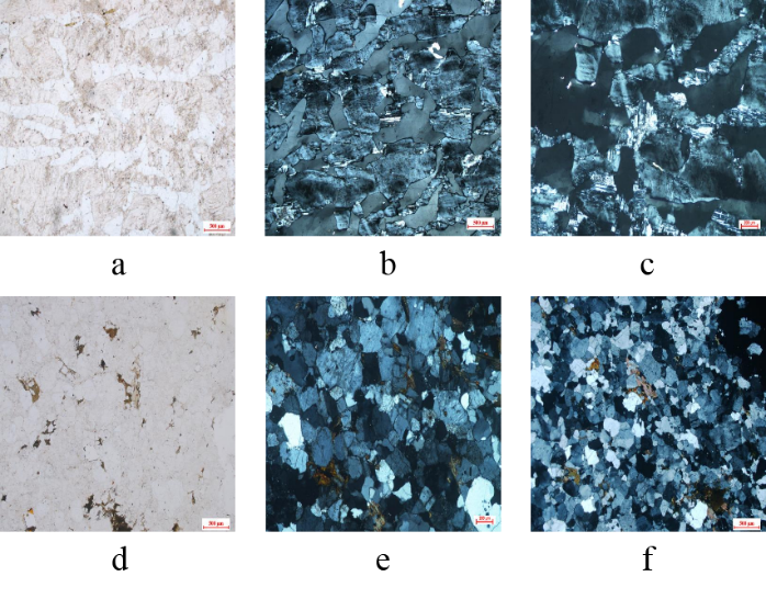
By analyzing the characteristics of misclassification, it can be seen that the sample distribution characteristics of pegmatite and granulite are highly similar. It can be seen from Figure 6 that the single polarized light photos of pegmatite (abc) and granulite (def) are light white and in the shape of spots. The reason for this error is that the blue cross polarization image with the characteristics of regional block structure causes a certain degree of interference, which tends to produce errors. Experienced experts can distinguish these similarities by observing the specific features of the image, and the neural network may make wrong recognition according to the similar sample distribution.
# Define training process
iters_list=[]
train_acc_list=[]
train_loss_list=[]
val_acc_list=[]
triplet_loss_list=[]
val_acc=0
iters = 0

def train_pm(model, optimizer):
    # Turn on GPU training
    use_gpu = True
    paddle.set_device('gpu') if use_gpu else paddle.set_device('cpu')
    epoch_num = 140
    global iters_list
    global train_acc_list
    global train_loss_list
    global val_acc_list
    global triplet_loss_list
    global val_acc
    global iters
    for epoch in range(epoch_num):
        for batch_id, data in enumerate(triloss_loader()):
            model.train()
            x_data, y_data = data
            #print(x_data.shape,y_data.shape,y_data)
            img = paddle.to_tensor(x_data)
            label = paddle.to_tensor(y_data) #[32, 1]
            #print(img,label)
            # Run the forward calculation of the model to obtain the predicted value
            feature2048,logits = model(img) #[32, 751]

            #triplet_loss=Trihard_loss(feature2048,label,num_identities=16,num_instances=4)
            #################
            triplet_loss=batch_hard_triplet_loss(feature2048, label, 0.8,64)
            ###################

            loss = F.softmax_with_cross_entropy(logits, label)
            #print(loss.shape)
            avg_loss = paddle.mean(loss)
            loss_all=avg_loss+triplet_loss
            #print('avg_loss: ',avg_loss,'avg_triplet_loss: ',avg_triplet_loss)
            acc = paddle.metric.accuracy(logits, label)
            avg_acc=paddle.mean(acc)
            if batch_id % 10 == 0:
                print("epoch: {}, batch_id: {}, <classifyloss is: {}>,  <Triple_loss is:{}>,  <classify_acc is: {}>".format(epoch, batch_id, avg_loss.numpy(),triplet_loss.numpy(),avg_acc.numpy()))
                #print('P:',positive_loss,'N:',negtive_loss)
                log_writer.add_scalar(tag = 'train_acc', step = iters, value = avg_acc.numpy())
                log_writer.add_scalar(tag = 'train_loss', step = iters, value = avg_loss.numpy())
                log_writer.add_scalar(tag = 'triloss', step = iters, value = triplet_loss.numpy())
                log_writer.add_histogram(tag='logits',values=logits.numpy(),step=iters,buckets=5)
                log_writer.add_histogram(tag='feature2048',values=feature2048.numpy(),step=iters,buckets=30)
                iters += 10
                iters_list.append([iters])
                train_acc_list.append(avg_acc.numpy())
                train_loss_list.append(avg_loss.numpy())
                triplet_loss_list.append(triplet_loss.numpy())
                val_acc_list.append([val_acc])
            # Back propagation, update weight, clear gradient
            loss_all.backward()
            #print('avg_loss.grad: ',avg_loss.grad,'triplet_loss.grad: ',triplet_loss.grad,'feature2048.grad: ',feature2048.grad,'loss_all.grad: ',loss_all.grad,'logits.grad: ',logits.grad)
            optimizer.step()
            optimizer.clear_grad()
        model.eval()
        accuracies = []
        losses = []
        for batch_id, data in enumerate(val_loader()):
            x_data, y_data = data
            img = paddle.to_tensor(x_data)
            label = paddle.to_tensor(y_data)
            # Run the forward calculation of the model to obtain the predicted value
            feature2048,logits = model(img)
            #print(logits)
            #print('logits : ',logits.shape)
            # Calculate the prediction probability after sigmoid and calculate the loss
            pred = F.softmax(logits)
            loss = F.softmax_with_cross_entropy(logits, label)
            acc = paddle.metric.accuracy(pred, label)
            #print('pred = {},loss = {},acc = {}'.format(pred.shape,loss.shape,acc.shape))
            accuracies.append(acc.numpy())
            losses.append(np.mean(loss.numpy()))
        #accuracies=np.array(accuracies)
        val_acc=np.mean(accuracies)
        lossess=np.mean(np.array(losses).reshape([-1,1]))
        #print('accuracies = {},losses = {}'.format(accuracies.shape,losses.shape))
        print("$$-val>>>>>>  <loss is: {}>,  <acc is: {}>".format(lossess,val_acc))
        paddle.save(model.state_dict(), 'palm.pdparams')
        paddle.save(optimizer.state_dict(), 'palm.pdopt')
summary
The identification of rock thin sections is indispensable in the process of oil and gas exploration and development. We realize high-precision automatic lithofacies analysis based on flying propeller, help the exploration and development design of oil and gas fields, and liberate scientific researchers from repeated work.
On the one hand, the implementation of this project serves as the solution of rock thin section, on the other hand, it also serves as the migration basis of oil and gas industry, and provides an extensible scheme for many problems under the background of cross source large-scale
Source: [1] he ma, et al., 2021 Rock thin sections identification based on improved squeeze-and-Excitation Networks model[J] Comput. Geosci. one hundred and fifty-two
Operating environment: https://aistudio.baidu.com/aistudio/projectdetail/1876529?channelType=0&channel=0