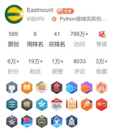
It has been ten years since I came to CSDN in 2010 and wrote my first blog in 2013. 590 original articles, 7.86 million times of reading and 190000 followers. Behind these numbers, I paid silently for more than 3000 days and made efforts to write nearly 10 million words.
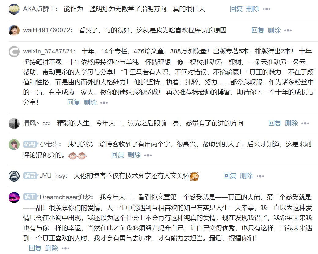
Some people say that everything in the world is met and chance. Yes, because of CSDN, I have become good friends with many people. Although I haven't met, it feels good to silently encourage and share with each other; Because of CSDN, many stories of one eighth (ten years) of my life progress bar are written here, and I can't live up to time; Because of CSDN, I cherish every blogger, friend and teacher, answer your questions, and encourage those who fail to take the postgraduate entrance examination or find a job to continue to fight; Because of CSDN, I met the goddess and shared many stories of our family.
The night of Dongxi Lake is very quiet, the doctor's journey is very hard, and his relatives in the distance miss him very much.
Why should I write such an article? On the one hand, I would like to thank the readers for their company and tolerance in the past ten years. No matter what I share, you have given me encouragement and moved; On the other hand, because of the change, I will bid farewell to CSDN for a short time (the technology update slows down) and settle down to read papers and do scientific research.
At the same time, this article is very hard core. It will use Python text mining to share the stories of this decade in detail. It can also be regarded as some benefits for beginners of text mining and readers who write relevant papers. Sincerely say thank you to everyone, thank you for your ten years of company, live up to your meeting and time. Please remember that a sharer named Eastmount is enough for this life~
I Recalling the past and sharing the years
For the story of the author and CSDN in the past ten years, you can read this article:
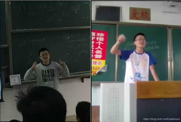
Ten years, fleeting, I grew up from a green boy to a middle-aged uncle. Maybe blogging is plain for others, but for me, it may be one of the most important decisions and stick to in my decade.
Ten years, no, no, no, no, no, No. I am grateful for everyone's company, because with you, I am not alone on the road of life. Fortunately, over the past ten years, I can touch my conscience and say that I am seriously writing and carving every blog, and I am full of blood in ten thousand words.
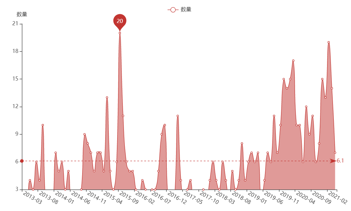
The following figure shows the monthly statistics of the number of sharing blogs in the past ten years. From finding a job in 2015 to reading a blog now, learning safety knowledge and sharing from zero is another peak.
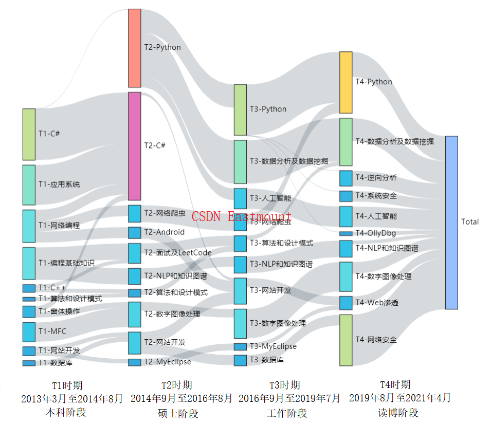
The following figure shows the Theme Evolution of my blog in CSDN in the past decade. In the whole decade, I have experienced four stages.
- Undergraduate stage: March 2013 to August 2014
At that time, undergraduate courses were the main courses, including C#, network development, basic course knowledge and so on. - Master's degree: September 2014 to August 2016
At this stage, the postgraduate direction is NLP and knowledge map, so they have written a lot of basic knowledge of Python, including Android, C#, interview, LeetCode, website development and so on. - Work phase: September 2016 to July 2019
At this stage, the author first entered the workplace, chose to return to Guizhou as an ordinary university teacher, shared courses such as Python data mining and website development, and wrote columns such as Python artificial intelligence and python image processing. - PhD stage: September 2019 to April 2021
At this stage, the author returned to the campus again, left his hometown relatives, chose to read a blog, and changed the general direction to learn system security and network security. A large amount of security knowledge was learned from scratch. The columns of network security self-study, network security improvement class and system security and malicious code detection were also opened.
Many people ask me, "do you share happiness?"
Happy. In fact, every time I write a blog, I am very happy. Every time I see a praise or comment from readers, I am really happy like a child.
Then why disappear for a short time?
Because of graduation, because of homesickness, because of missing him (her). I believe that most sharers are in the same mood as me. The charm of sharing knowledge is unforgettable for a long time. However, each stage needs to be done, especially the distant relatives. After my repeated thinking, I decided to put down the writing of technical blog for a short time and choose thesis research instead.

A brief disappearance does not mean no sharing.
The next 90% of the sharing will be related to papers and scientific research technology, and no longer PUSH their own articles every month. I don't know what degree I can achieve in the next few years, and I can't guarantee whether I can send a high-quality paper, but I will fight, fight and enjoy. Besides, in the past ten years, I never think I am a smart person. There are too many people better than me. What I prefer is to write silently, experience silently and grow up with you. When others praised my blog, I replied more "it's all made in time", and it's really made in time. I just wrote it for 3012 days.
But I really enjoy it. I enjoy everything I share in CSDN, the meeting and acquaintance with every blogger, and the blessings and encouragement of every friend. I am grateful to write 590 articles, 65 columns, tens of millions of words and codes. I can barely say "live up to my meeting and youth, this life is enough".


The following figure shows the various directions of my blog in the past decade. Over the years, I have always known that I have learned too much, but not in-depth. I hope to go deep into a certain field during my PhD. I have also learned a lot of basic safety knowledge, so it is time to enter the fifth stage and start the reading and writing of papers and the reproduction of experiments. I also hope the bloggers understand and look forward to your company.
Sand can't be held, so can time.
But when I pay, I can lift it up easily, and I can record what happens in time, such as technology and love. Is it hard to read a blog? Bitter, countless silent nights need us to endure and fight, but some people are more bitter, such as another at home. For the next three years, I hope I will always remember why I chose to come here and Dongxi Lake. It's also time to settle down to study papers and experiments. It's time to let go of technology sharing, although I don't give up. If you can't hold the sand, raise it easily; Even if I return to the origin, I haven't lost anything. Moreover, this experience is also the talk of life. I also hope that every blogger will cherish the present, do what they like and experience.
I looked at the road. The entrance of the dream was a little narrow, which was perhaps the most beautiful accident.
I will use this article in the first mass distribution of CSDN. Please forgive me. The next time should be the day of my doctoral graduation in 2024. Thanks again for everyone's company. A good sharer needs to constantly learn new knowledge and summarize cutting-edge technologies to everyone, so we should respect the fruits of every creator. At the same time, I am here to assure all readers that in three years, I will share better articles with new understanding and new feelings, give back to all readers and help more beginners get started. Maybe I will write a very detailed summary.
Thank you again. I hope you will remember that CSDN has an author named Eastmount and a blogger named Yang xiuzhang. If you can remember Nazhang and Xiaoluo's family, you will be happier. Ha ha ~ love you. Readers who are confused or encounter difficulties can join me in wechat to move forward together.

Our stories are still being written, and your company continues.
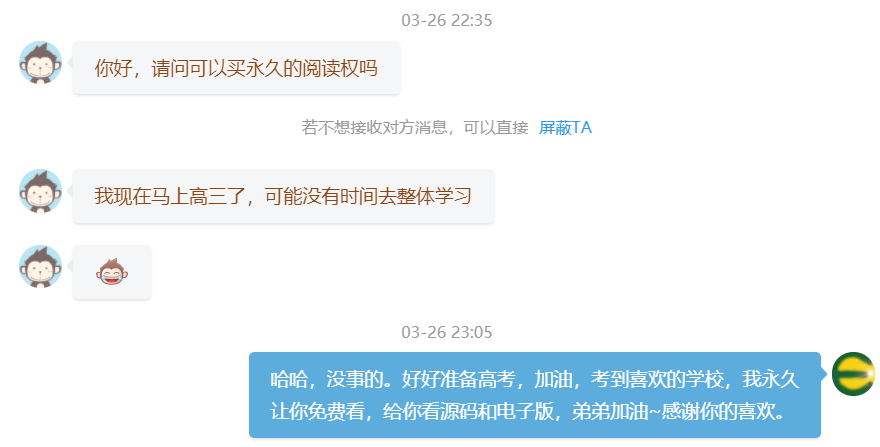
Finally, readers familiar with me know that I have opened three paid columns. There are often readers who are in school or have financial difficulties, so I mentioned many times in my article that I can talk about the full text privately. In fact, I have already opened these articles to github. I hope every reader can learn knowledge from the articles. I hope that the articles are good and easy to give a reward of 9 yuan. The milk powder money is enough. Here, I also share these three addresses with readers in need! And line and cherish, purchase is also welcome.
- Python image processing
https://github.com/eastmountyxz/CSDNBlog-ImageProcessing - Network security self study
https://github.com/eastmountyxz/CSDNBlog-Security-Based - Python artificial intelligence
https://github.com/eastmountyxz/CSDNBlog-AI-for-Python
Say sorry to those who want to learn technology. Remember to wait for me! See you in the Jianghu. Thank you for coming.

II Hard core CSDN blog text mining
Before, I gave a wave of benefits to readers who study safety and told you the safe learning route and CSDN excellent bloggers.
Here, I'll finally give Python text mining readers a wave of benefits. I hope you like ~ the idea of this article. You can learn from it, but don't take it directly to write a paper! But the idea is very clear. You must write the code.
1. Data crawling
The specific code will not be introduced here to protect the original CSDN, but the corresponding core knowledge points will be given. Readers are advised to grasp the text knowledge in combination with their own direction.
Core expansion pack:
- import requests
- from lxml import etree
- import csv
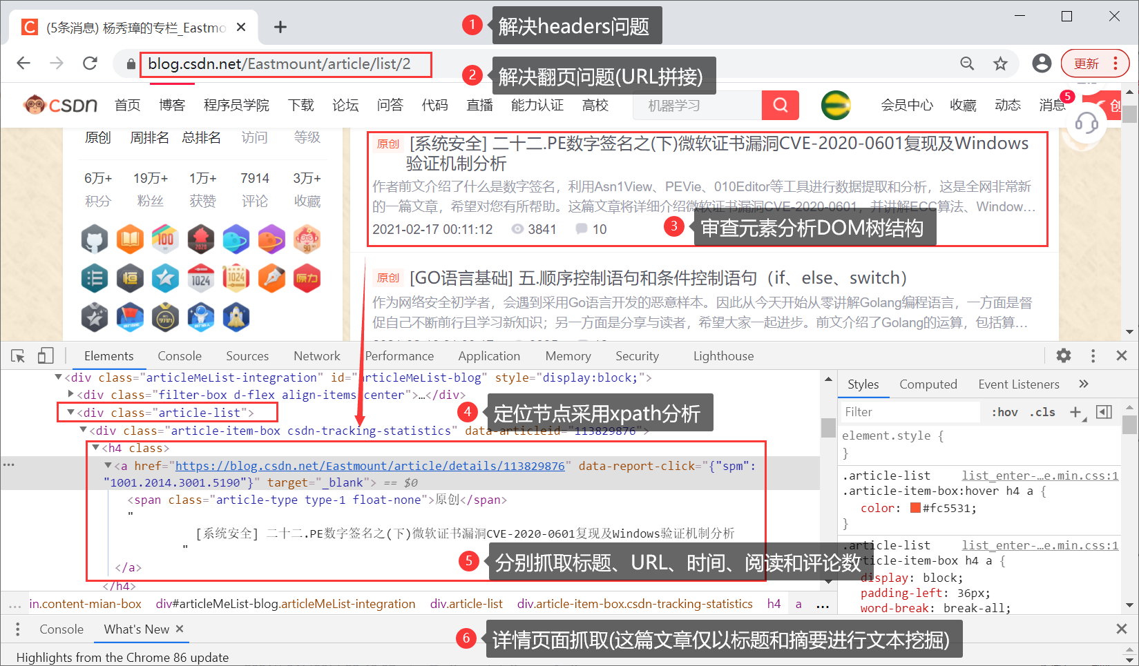
Core process:
- Solve the header problem
- Solve page turning problem
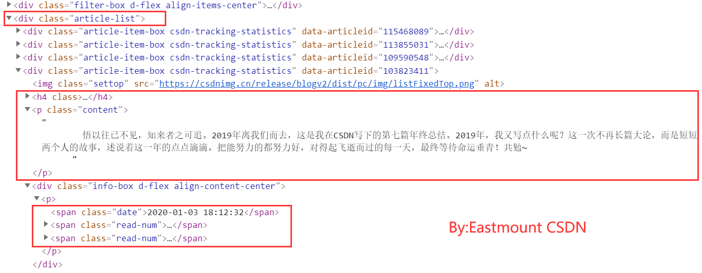
- Review element analysis DOM tree structure
- The positioning node is analyzed by Xpath
- Earn titles, URL s, times, readings and comments respectively
- Detail page capture
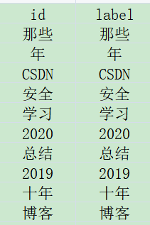
Crawler output results, it is recommended to learn pile driving output (multi-purpose print).
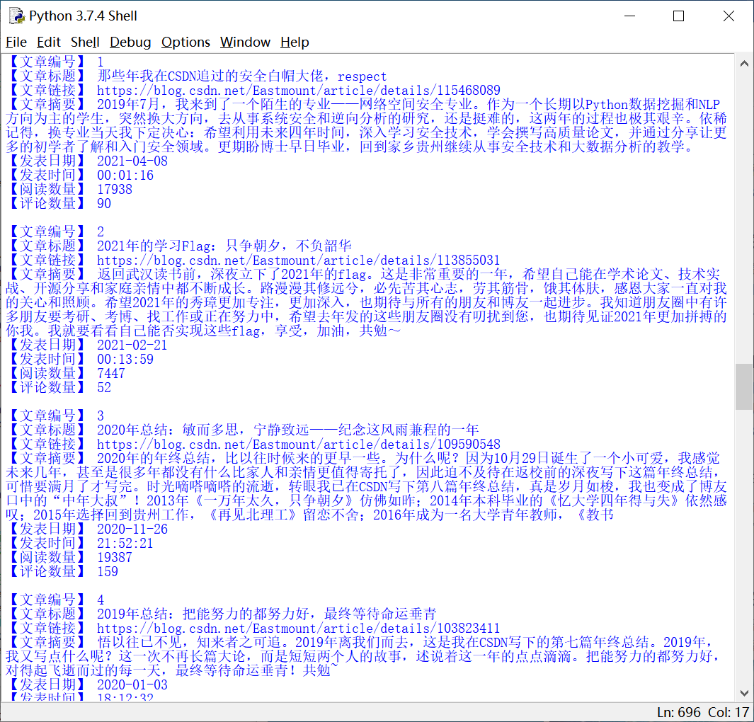
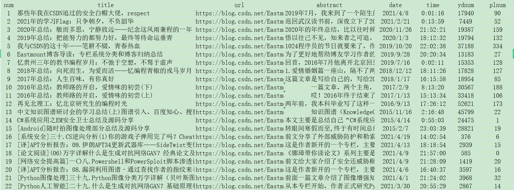
The sorted results are shown in the figure below, and the contents are output to CSV storage.
2. Metrological statistics and visual analysis
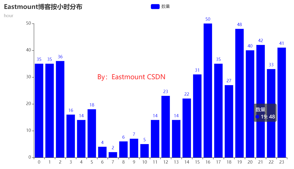
(1) Analyze the author's writing habits by hour
First, let's analyze the blog writing habits of the author "Eastmount". At the same time, we use Matplotlib and pyecarts to draw graphics. We find that the graphics drawn by ecarts are more beautiful. As can be seen from the figure, the author has been writing blogs late at night and in the afternoon for a long time.
The source code is as follows:
# encoding:utf-8
"""
By: Easmount CSDN 2021-04-19
"""
import re
import time
import csv
import pandas as pd
import numpy as np

#------------------------------------------------------------------------------
#Step 1: read data
dd = []   #date
tt = []   #time
with open("data.csv", "r", encoding="utf8") as csvfile:
    csv_reader = csv.reader(csvfile)
    k = 0
    for row in csv_reader:
        if k==0:      #Skip title
            k = k + 1
            continue
        #Get data 2021-04-08 21:52:21
        value_date = row[4]
        value_time = row[5]
        hour = value_time.split(":")[0]
        hour = int(hour)
        dd.append(row[4])
        tt.append(hour)
        #print(row[4],row[5])
        #print(hour)
        k = k + 1
print(len(tt),len(dd))
print(dd)
print(tt)

#------------------------------------------------------------------------------
#The second step is to count the number of different hours
from collections import Counter
cnt = Counter(tt)
print(cnt.items())  #dict_items
#Dictionary key sorting
list_time = []
list_tnum = []
for i in sorted(cnt):
    print(i,cnt[i])
    list_time.append(i)
    list_tnum.append(cnt[i])

#------------------------------------------------------------------------------
#Step 3 draw a histogram
import matplotlib.pyplot as plt
N = 24
ind = np.arange(N)
width=0.35
plt.bar(ind, list_tnum, width, color='r', label='hour')
plt.xticks(ind+width/2, list_time, rotation=40)
plt.title("The Eastmount's blog is distributed by the hour")
plt.xlabel('hour')
plt.ylabel('numbers')
plt.savefig('Eastmount-01.png',dpi=400)
plt.show()

#------------------------------------------------------------------------------
#Step 4: PyEcharts draw histogram

from pyecharts import options as opts
from pyecharts.charts import Bar
bar=(
    Bar()
        .add_xaxis(list_time)
        .add_yaxis("quantity", list_tnum, color="blue")
        .set_global_opts(title_opts=opts.TitleOpts(
            title="Eastmount Blogs are distributed by hour", subtitle="hour"))
    )
bar.render('01-Eastmount Blogs are distributed by hour.html')
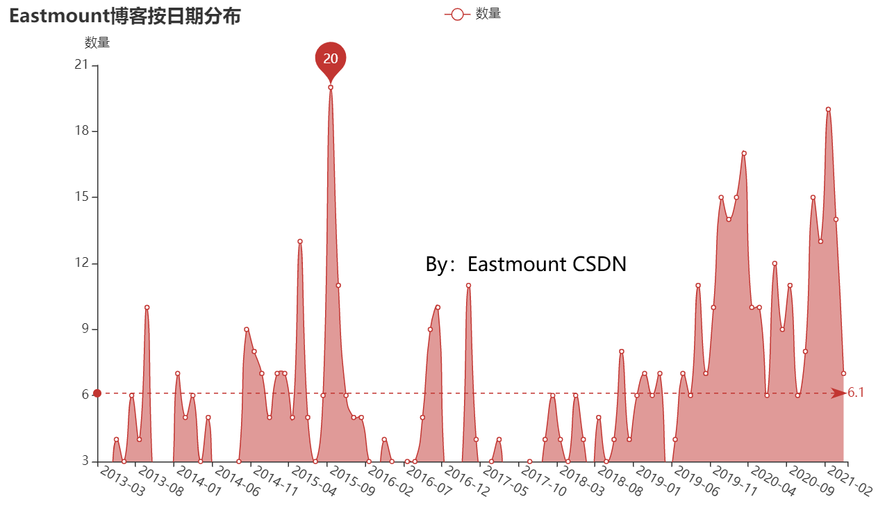
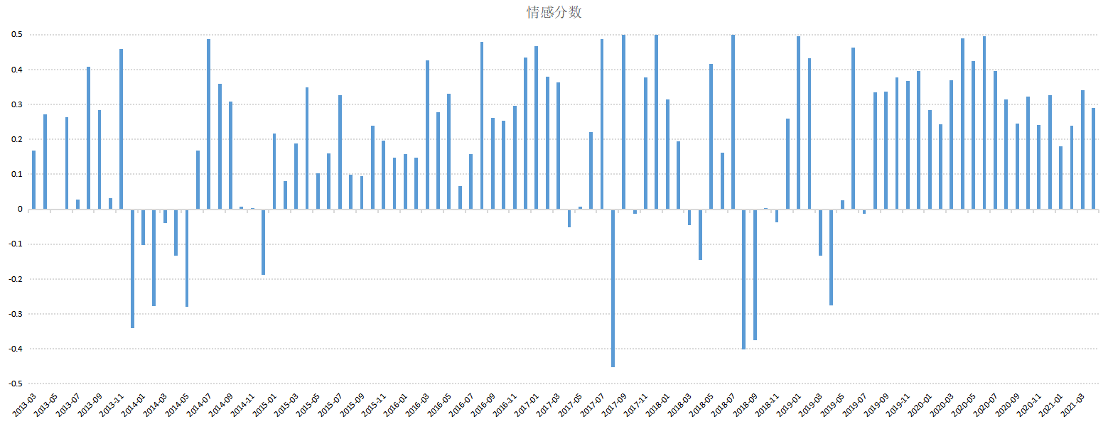
(2) Blog statistics by month
The author writes a blog by month, as shown in the figure below. In 2015, he wrote a lot of LeetCode code when looking for a job. Later, he shared more security during his blog reading.
The source code is as follows:
# encoding:utf-8
"""
By: Easmount CSDN 2021-04-19
"""
import re
import time
import csv
import pandas as pd
import numpy as np

#------------------------------------------------------------------------------
#Step 1: read data
dd = []   #date
tt = []   #time
with open("data.csv", "r", encoding="utf8") as csvfile:
    csv_reader = csv.reader(csvfile)
    k = 0
    for row in csv_reader:
        if k==0:      #Skip title
            k = k + 1
            continue
        #Get data 2021-04-08 21:52:21
        value_date = row[4]
        value_time = row[5]
        hour = value_time.split(":")[0]   #Get hours
        hour = int(hour)
        month = value_date[:7]            #Get month
        dd.append(month)
        tt.append(hour)
        #print(row[4],row[5])
        #print(hour,month)
        print(month)
        k = k + 1
        #break
print(len(tt),len(dd))
print(dd)
print(tt)

#------------------------------------------------------------------------------
#Step 2: count the number of different dates
from collections import Counter
cnt = Counter(dd)
print(cnt.items())  #dict_items
#Dictionary key sorting
list_date = []
list_dnum = []
for i in sorted(cnt):
    print(i,cnt[i])
    list_date.append(i)
    list_dnum.append(cnt[i])

#------------------------------------------------------------------------------
#Step 3: PyEcharts draw a histogram
from pyecharts import options as opts
from pyecharts.charts import Bar
from pyecharts.charts import Line
from pyecharts.commons.utils import JsCode

line = (
    Line()
    .add_xaxis(list_date)
    .add_yaxis('quantity', list_dnum, is_smooth=True,
               markline_opts=opts.MarkLineOpts(data=[opts.MarkLineItem(type_="average")]),
               markpoint_opts=opts.MarkPointOpts(data=[opts.MarkPointItem(type_="max"),
                                                       opts.MarkPointItem(type_="min")]))
    # Hide numbers set area
    .set_series_opts(
        areastyle_opts=opts.AreaStyleOpts(opacity=0.5),
        label_opts=opts.LabelOpts(is_show=False))
    # Sets the rotation angle of the x-axis label
    .set_global_opts(xaxis_opts=opts.AxisOpts(axislabel_opts=opts.LabelOpts(rotate=-30)),
                     yaxis_opts=opts.AxisOpts(name='quantity', min_=3),
                     title_opts=opts.TitleOpts(title='Eastmount Blog distribution by date'))
    )
line.render('02-Eastmount Blog distribution by date.html')
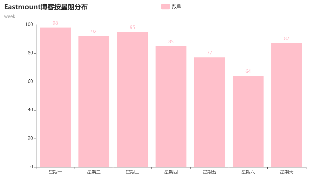
(3) Blog statistics by week
Statistics by week are as follows: call date The weekday () function can output the corresponding week. The author updates a little less at the weekend.
The core code is as follows:
# encoding:utf-8
"""
By: Easmount CSDN 2021-04-19
"""
import re
import time
import csv
import pandas as pd
import numpy as np
import datetime

#Define week function
def get_week_day(date):
    week_day_dict = {
        0 : 'Monday',
        1 : 'Tuesday',
        2 : 'Wednesday',
        3 : 'Thursday',
        4 : 'Friday',
        5 : 'Saturday',
        6 : 'Sunday'
    }
    day = date.weekday()
    return week_day_dict[day]

#------------------------------------------------------------------------------
#Step 1: read data

dd = []   #date
tt = []   #time
ww = []   #week
with open("data.csv", "r", encoding="utf8") as csvfile:
    csv_reader = csv.reader(csvfile)
    k = 0
    for row in csv_reader:
        if k==0:      #Skip title
            k = k + 1
            continue
        #Get data 2021-04-08 21:52:21
        value_date = row[4]
        value_time = row[5]
        hour = value_time.split(":")[0]   #Get hours
        hour = int(hour)
        month = value_date[:7]            #Get month
        dd.append(month)
        tt.append(hour)

        #Get week
        date = datetime.datetime.strptime(value_date, '%Y-%m-%d').date()
        week = get_week_day(date)
        ww.append(week)
        #print(date,week)
        k = k + 1
print(len(tt),len(dd),len(ww))
print(dd)
print(tt)
print(ww)

#------------------------------------------------------------------------------
#Step 2: count the number of different dates
from collections import Counter
cnt = Counter(ww)
print(cnt.items())  #dict_items
#Dictionary key sorting
list_date = ['Monday','Tuesday','Wednesday','Thursday','Friday','Saturday','Sunday']
list_dnum = [0,0,0,0,0,0,0]

for key,value in cnt.items():
    k = 0
    while k<len(list_date):
        if key==list_date[k]:
            list_dnum[k] = value
            break
        k = k + 1
print(list_date,list_dnum)

#------------------------------------------------------------------------------
#Step 3: PyEcharts draw a histogram
from pyecharts import options as opts
from pyecharts.charts import Bar
from pyecharts.charts import Line
from pyecharts.commons.utils import JsCode
bar=(
    Bar()
        .add_xaxis(list_date)
        .add_yaxis("quantity", list_dnum, color='pink')
        .set_global_opts(title_opts=opts.TitleOpts(
            title="Eastmount Blogs by week", subtitle="week"))
    )
bar.render('03-Eastmount Blogs by week.html')
3. Core word statistics and word cloud analysis
Word cloud analysis is very suitable for beginners. Here, the author also briefly shares the process of core topic word statistics and word cloud analysis.
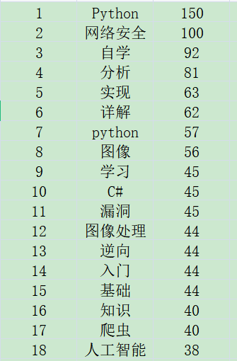
(1) Statistical core keywords and word frequency
The output results are shown in the figure below:
The code is as follows:
# coding=utf-8
"""
By: Easmount CSDN 2021-04-19
"""
import jieba
import re
import time
import csv
from collections import Counter

#------------------------------------Chinese word segmentation----------------------------------
cut_words = ""
all_words = ""
stopwords = ["[", "]", ")", "(", ")", "(", "[", "]",
             ".", ",", "-", "—", ":", ": ", "<", ">",
             "of", "and", "of", "and", """, """, "?", "?"]

#Import custom dictionary
#jieba.load_userdict("dict.txt")

f = open('06-data-fenci.txt', 'w')

with open("data.csv", "r", encoding="utf8") as csvfile:
    csv_reader = csv.reader(csvfile)
    k = 0
    for row in csv_reader:
        if k==0:      #Skip title
            k = k + 1
            continue
        #get data
        title = row[1]
        title = title.strip('\n')
        #print(title)
        #participle
        cut_words = ""
        seg_list = jieba.cut(title,cut_all=False)
        for seg in seg_list:
            if seg not in stopwords:
                cut_words += seg + " "
        #cut_words = (" ".join(seg_list))
        f.write(cut_words+"\n")
        all_words += cut_words
        k = k + 1
f.close()
#Output results
all_words = all_words.split()
print(all_words)

#------------------------------------Word frequency statistics----------------------------------
c = Counter()
for x in all_words:
    if len(x)>1 and x != '\r\n':
        c[x] += 1
#Output the top 10 words with the highest word frequency
print('\n Statistical results of word frequency:')
for (k,v) in c.most_common(10):
    print("%s:%d"%(k,v))
#Store data
name ="06-data-word.csv"
fw = open(name, 'w', encoding='utf-8')
i = 1
for (k,v) in c.most_common(len(c)):
    fw.write(str(i)+','+str(k)+','+str(v)+'\n')
    i = i + 1
else:
    print("Over write file!")
    fw.close()
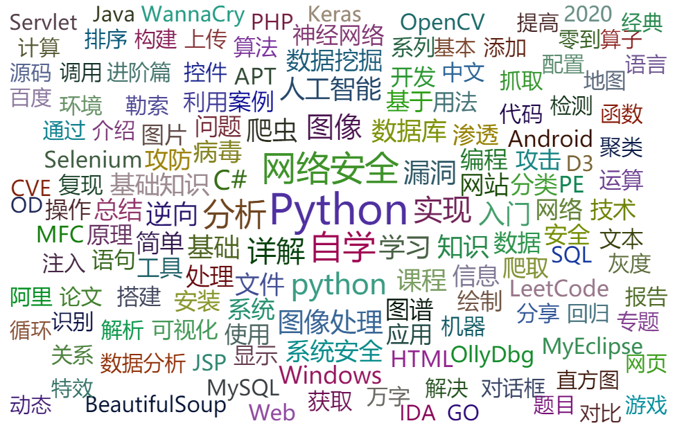
(2) PyEcharts word cloud visualization
The output results are shown in the figure below. The words with higher word frequency are displayed larger and brighter.
The code is as follows:
# coding=utf-8
"""
By: Easmount CSDN 2021-04-19
"""
import jieba
import re
import time
import csv
from collections import Counter

#------------------------------------Chinese word segmentation----------------------------------
cut_words = ""
all_words = ""
stopwords = ["[", "]", ")", "(", ")", "(", "[", "]",
             "01", "02", "03", "04", "05", "06", "07",
             "08", "09", "what"]
f = open('06-data-fenci.txt', 'w')

with open("data.csv", "r", encoding="utf8") as csvfile:
    csv_reader = csv.reader(csvfile)
    k = 0
    for row in csv_reader:
        if k==0:      #Skip title
            k = k + 1
            continue
        #get data
        title = row[1]
        title = title.strip('\n')
        #print(title)
        #participle
        cut_words = ""
        seg_list = jieba.cut(title,cut_all=False)
        for seg in seg_list:
            if seg not in stopwords:
                cut_words += seg + " "
        #cut_words = (" ".join(seg_list))
        f.write(cut_words+"\n")
        all_words += cut_words
        k = k + 1
f.close()
#Output results
all_words = all_words.split()
print(all_words)

#------------------------------------Word frequency statistics----------------------------------
c = Counter()
for x in all_words:
    if len(x)>1 and x != '\r\n':
        c[x] += 1
#Output the top 10 words with the highest word frequency
print('\n Statistical results of word frequency:')
for (k,v) in c.most_common(10):
    print("%s:%d"%(k,v))
#Store data
name ="06-data-word.csv"
fw = open(name, 'w', encoding='utf-8')
i = 1
for (k,v) in c.most_common(len(c)):
    fw.write(str(i)+','+str(k)+','+str(v)+'\n')
    i = i + 1
else:
    print("Over write file!")
    fw.close()

#------------------------------------Word cloud analysis----------------------------------
from pyecharts import options as opts
from pyecharts.charts import WordCloud
from pyecharts.globals import SymbolType

# Generate data word = [('A',10), ('B',9), ('C',8)] list + Tuple
words = []
for (k,v) in c.most_common(200):
    # print(k, v)
    words.append((k,v))
# Rendering
def wordcloud_base() -> WordCloud:
    c = (
        WordCloud()
        .add("", words, word_size_range=[20, 40], shape='diamond') #shape=SymbolType.ROUND_RECT
        .set_global_opts(title_opts=opts.TitleOpts(title='Eastmount Ten year blog word cloud map'))
    )
    return c

# Generate graph
wordcloud_base().render('05-Eastmount Ten year blog word cloud map.html')
4.LDA theme mining
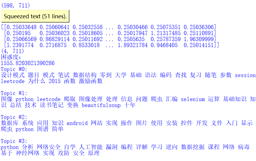
LDA model is a very classic algorithm in text mining or topic mining. Readers can read the author's previous articles and introduce the model in detail. Here, we use it to mine the theme of the author's blog. The number of topics set is 4. It is usually necessary to calculate the confusion comparison.
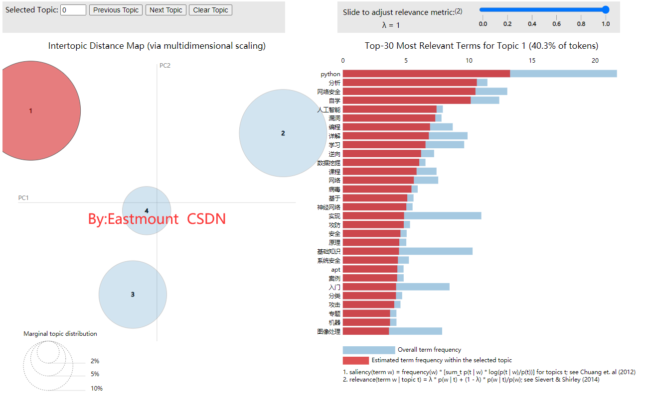
At the same time, calculate the subject words corresponding to each subject, as shown below. For example, the theme of Python series will be optimized, and readers will pay more attention to the integration of their own themes, which will be more relevant to each other. For example, the theme of Python series will be optimized, and readers will pay more attention to each other.
The complete code is as follows:
#coding: utf-8
import pandas as pd
from sklearn.feature_extraction.text import TfidfVectorizer, CountVectorizer

#---------------------Step 1: read data (word segmentation)----------------------
corpus = []

# One line of read is expected to be one document
for line in open('06-data-fenci.txt', 'r').readlines():
    corpus.append(line.strip())

#-----------------------Step 2: calculate TF-IDF value-----------------------
# Set the number of features
n_features = 2000
tf_vectorizer = TfidfVectorizer(strip_accents = 'unicode',
                                max_features=n_features,
                                stop_words=['of','or','etc.','yes','have','of','And','sure','still','here',
                                            'One','and','also','cover','Do you','to','in','most','however','everybody',
                                            'once','How many days?','200','also','A look','300','50','Ha ha ha ha',
                                             '"','"','. ',',','?',',',';','Yes?','originally','find',
                                             'and','in','of','the','We','always','really','18','once',
                                           'Yes','Some','already','no','such','one by one','one day','this','such',
                                           'one kind','be located','one of','sky','No,','quite a lot','somewhat','what','Five',
                                           'especially'],
                                max_df = 0.99,
                                min_df = 0.002) #Remove words that are too likely to appear in the document
tf = tf_vectorizer.fit_transform(corpus)
print(tf.shape)
print(tf)

#-------------------------Step 3 LDA analysis------------------------
from sklearn.decomposition import LatentDirichletAllocation
# Set number of topics
n_topics = 4
lda = LatentDirichletAllocation(n_components=n_topics,
                                max_iter=100,
                                learning_method='online',
                                learning_offset=50,
                                random_state=0)
lda.fit(tf)
# Show the number of topics model topic_ word_
print(lda.components_)
# Several topics are rows, and several keywords are columns
print(lda.components_.shape)
# Computational confusion
print(u'Confusion:')
print(lda.perplexity(tf,sub_sampling = False))

# Topic keyword distribution
def print_top_words(model, tf_feature_names, n_top_words):
    for topic_idx,topic in enumerate(model.components_):  # lda.component is equivalent to model topic_ word_
        print('Topic #%d:' % topic_idx)
        print(' '.join([tf_feature_names[i] for i in topic.argsort()[:-n_top_words-1:-1]]))
        print("")
# After defining the function, temporarily output the first 20 keywords for each topic
n_top_words = 20
tf_feature_names = tf_vectorizer.get_feature_names()
# Call function
print_top_words(lda, tf_feature_names, n_top_words)

#------------------------Step 4 visual analysis-------------------------
import pyLDAvis
import pyLDAvis.sklearn

#pyLDAvis.enable_notebook()
data = pyLDAvis.sklearn.prepare(lda,tf,tf_vectorizer)
print(data)
#display graphics
pyLDAvis.show(data)
pyLDAvis.save_json(data,' 06-fileobj.html')
5. Hierarchical clustering topic tree
The tree view drawn by hierarchical clustering is also a common technology in the field of text mining. It will display the topics related to each field in the form of tree. The output results here are shown in the following figure:
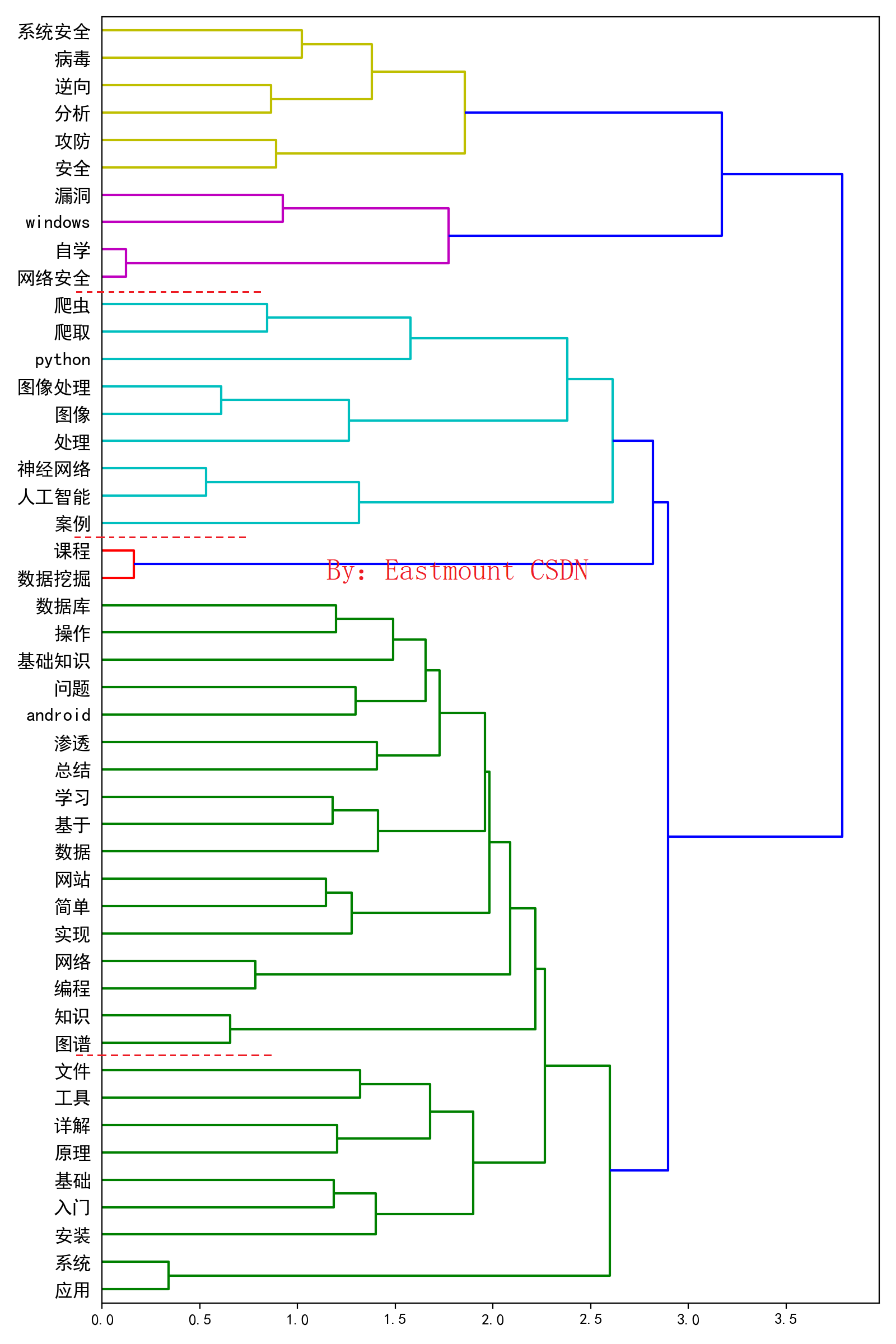
Note that here, the author can set filtering to display the number of subject words displayed in the tree view, and conduct relevant comparative experiments to find the best results.
# -*- coding: utf-8 -*-
import os
import codecs
from sklearn.feature_extraction.text import CountVectorizer, TfidfTransformer
from sklearn.manifold import TSNE
from sklearn.cluster import KMeans
import matplotlib.pyplot as plt
import numpy as np
import pandas as pd
import jieba
from sklearn import metrics
from sklearn.metrics import silhouette_score
from array import array
from numpy import *
from pylab import mpl
from sklearn.metrics.pairwise import cosine_similarity
import matplotlib.pyplot as plt
import matplotlib as mpl
from scipy.cluster.hierarchy import ward, dendrogram

#---------------------------------------Corpus loading-------------------------------------
text = open('06-data-fenci.txt').read()
print(text)
list1=text.split("\n")
print(list1)
print(list1[0])
print(list1[1])
mytext_list=list1

#Control the number of displays
count_vec = CountVectorizer(min_df=20, max_df=1000)  #Maximum ignored
xx1 = count_vec.fit_transform(list1).toarray()
word=count_vec.get_feature_names()
print("word feature length: {}".format(len(word)))
print(word)
print(xx1)
print(type(xx1))
print(xx1.shape)
print(xx1[0])

#---------------------------------------Hierarchical clustering-------------------------------------
titles = word
#dist = cosine_similarity(xx1)

mpl.rcParams['font.sans-serif'] = ['SimHei']

df = pd.DataFrame(xx1)
print(df.corr())
print(df.corr('spearman'))
print(df.corr('kendall'))
dist = df.corr()
print (dist)
print(type(dist))
print(dist.shape)

#define the linkage_matrix using ward clustering pre-computed distances
linkage_matrix = ward(dist)
fig, ax = plt.subplots(figsize=(8, 12)) # set size
ax = dendrogram(linkage_matrix, orientation="right",
                p=20, labels=titles, leaf_font_size=12
                ) #leaf_rotation=90., leaf_font_size=12.
#show plot with tight layout
plt.tight_layout()
#save figure as ward_clusters
plt.savefig('07-KH.png', dpi=200)
plt.show()
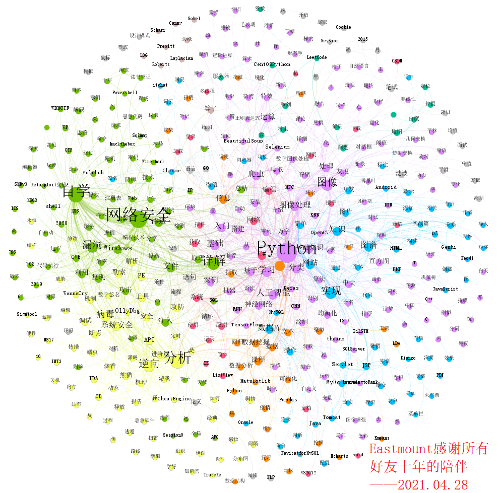
6. Social network analysis
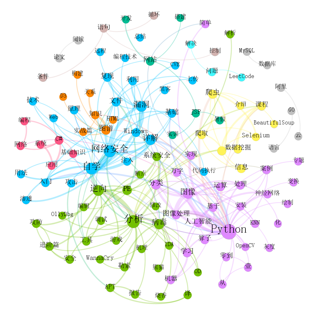
Social network analysis is often used in citation analysis. Some in the field of liberal arts become literature knowledge map (different from the knowledge map or ontology proposed by Google). It is also a common technical means in the field of literature mining. Here we draw the social network relationship map as shown below, mainly using Gephi software, and Neo4j or D3 is also recommended. It can be seen that the author's ten-year sharing mainly focuses on four pieces of content, which are interrelated and complement each other.
- network security
- Python
- backward analysis
- Basic knowledge or programming technology
Recommended articles:
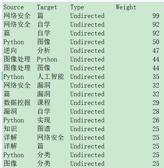
In the first step, we need to calculate the pairwise co-occurrence matrix. Too much data may overflow the boundary.
The output result is shown in the figure below. At this time, we hope you can filter the stop words or delete the abnormal relationship.
# -*- coding: utf-8 -*-
"""
@author: eastmount CSDN 2020-04-20
"""
import pandas as pd
import numpy as np
import codecs
import networkx as nx
import matplotlib.pyplot as plt
import csv
from scipy.sparse import coo_matrix

#---------------------------Step 1: read data-------------------------------
word = [] #Record keywords
f = open("06-data-fenci.txt", encoding='gbk')
line = f.readline()
while line:
    #print line
    line = line.replace("\n", "") #Filter line breaks
    line = line.strip('\n')
    for n in line.split(' '):
        #print n
        if n not in word:
            word.append(n)
    line = f.readline()
f.close()
print(len(word)) #Total number of keywords 2913

#--------------------------The second step is to calculate the co-occurrence matrix----------------------------
a = np.zeros([2,3])
print(a)

#Co-occurrence matrix
#word_vector = np.zeros([len(word),len(word)], dtype='float16')

#MemoryError: the matrix is too large. Coo is used to report memory errors_ The matrix function solves this problem
print(len(word))
#Type < type 'numpy ndarray'>
word_vector = coo_matrix((len(word),len(word)), dtype=np.int8).toarray()
print(word_vector.shape)

f = open("06-data-fenci.txt", encoding='gbk')
line = f.readline()
while line:
    line = line.replace("\n", "") #Filter line breaks
    line = line.strip('\n') #Filter line breaks
    nums = line.split(' ')

    #Cycle through the location of keywords and set word_vector count
    i = 0
    j = 0
    while i<len(nums):         #ABCD co existing AB AC AD BC BD CD plus 1
        j = i + 1
        w1 = nums[i]           #First word
        while j<len(nums):
            w2 = nums[j]       #Second word
            #Find the subscript corresponding to the word from the word array
            k = 0
            n1 = 0
            while k<len(word):
                if w1==word[k]:
                    n1 = k
                    break
                k = k +1
            #Find the second keyword location
            k = 0
            n2 = 0
            while k<len(word):
                if w2==word[k]:
                    n2 = k
                    break
                k = k +1
            #Key: the assignment of word frequency matrix only calculates the upper triangle
            if n1<=n2:
                word_vector[n1][n2] = word_vector[n1][n2] + 1
            else:
                word_vector[n2][n1] = word_vector[n2][n1] + 1
            #print(n1, n2, w1, w2)
            j = j + 1
        i = i + 1
    #Read new content
    line = f.readline()
    #print("next line")
f.close()
print("over computer")


#--------------------------Step 3: write CSV file--------------------------
c = open("word-word-weight.csv","w", encoding='utf-8', newline='')    #Solve blank lines
#c.write(codecs.BOM_UTF8)                                 #Prevent garbled code
writer = csv.writer(c)                                    #Write object
writer.writerow(['Word1', 'Word2', 'Weight'])

i = 0
while i<len(word):
    w1 = word[i]
    j = 0
    while j<len(word):
        w2 = word[j]
        #Judge whether two words co-exist. Write files with co-occurrence frequency not 0
        if word_vector[i][j]>0:
            #write file
            templist = []
            templist.append(w1)
            templist.append(w2)
            templist.append(str(int(word_vector[i][j])))
            #print templist
            writer.writerow(templist)
        j = j + 1
    i = i + 1
c.close()
In the second step, we need to build CSV files of entities (nodes) and relationships (edges). As shown in the figure below:
- entity-clean.csv
- rela-clean.csv
The third step is to create a new project, select "data" and enter the spreadsheet. Import the node table and select the entity table.
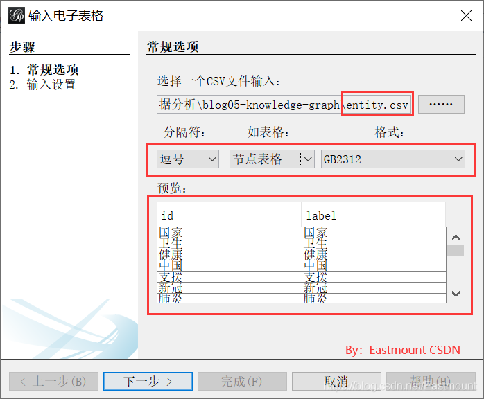
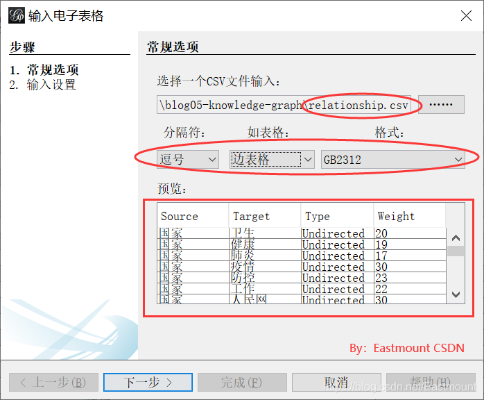
Step 4: import the data and set it as "edge table". Note that the CSV table data must be set as Source, Target and Weight. This must be consistent with the Gephi format, otherwise the imported data will prompt an error.
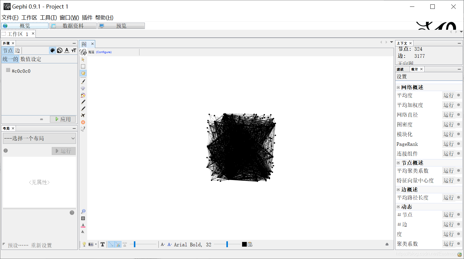
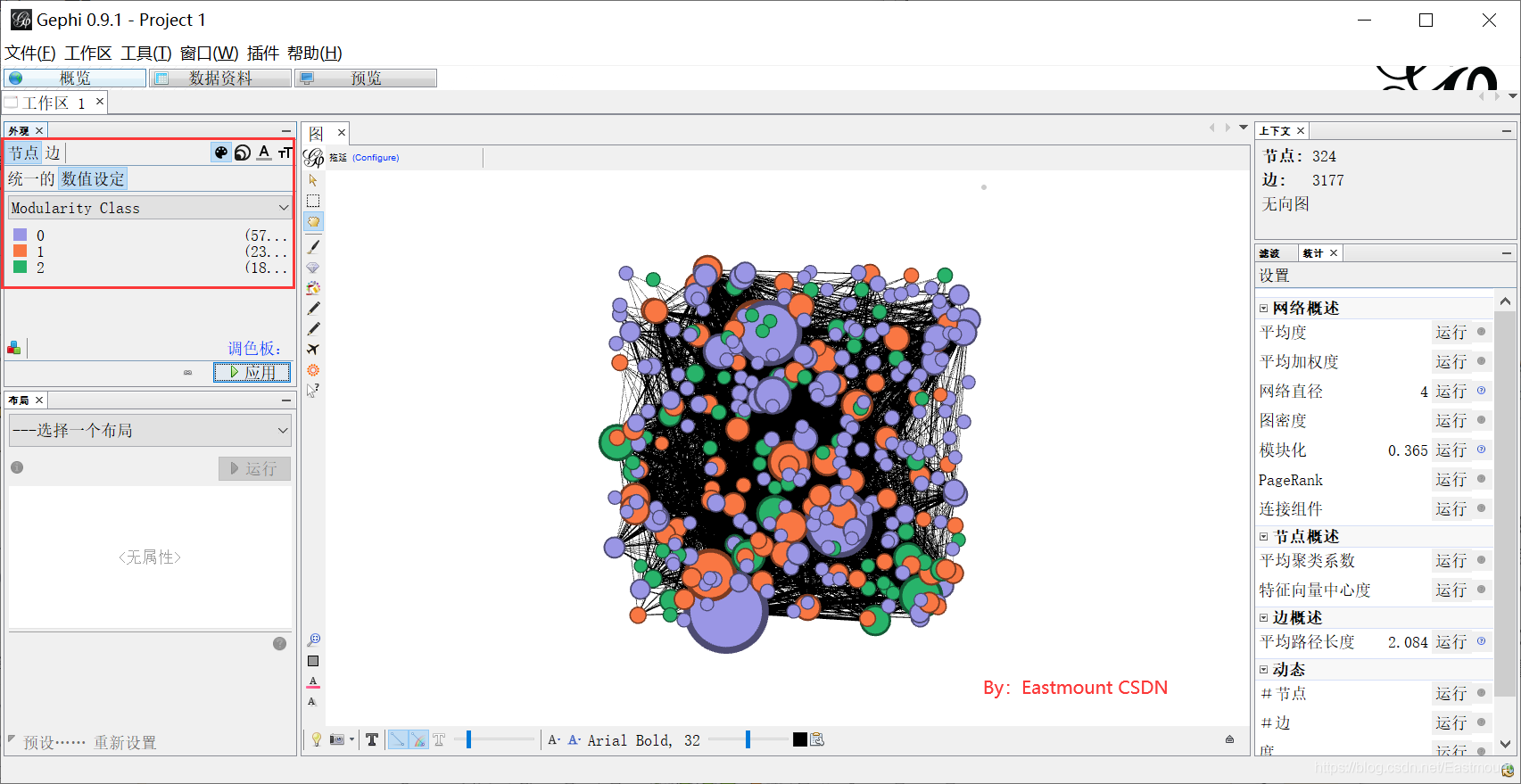
Step 5: after the import is successful, click "Overview" to display as shown below, and then adjust the parameters.
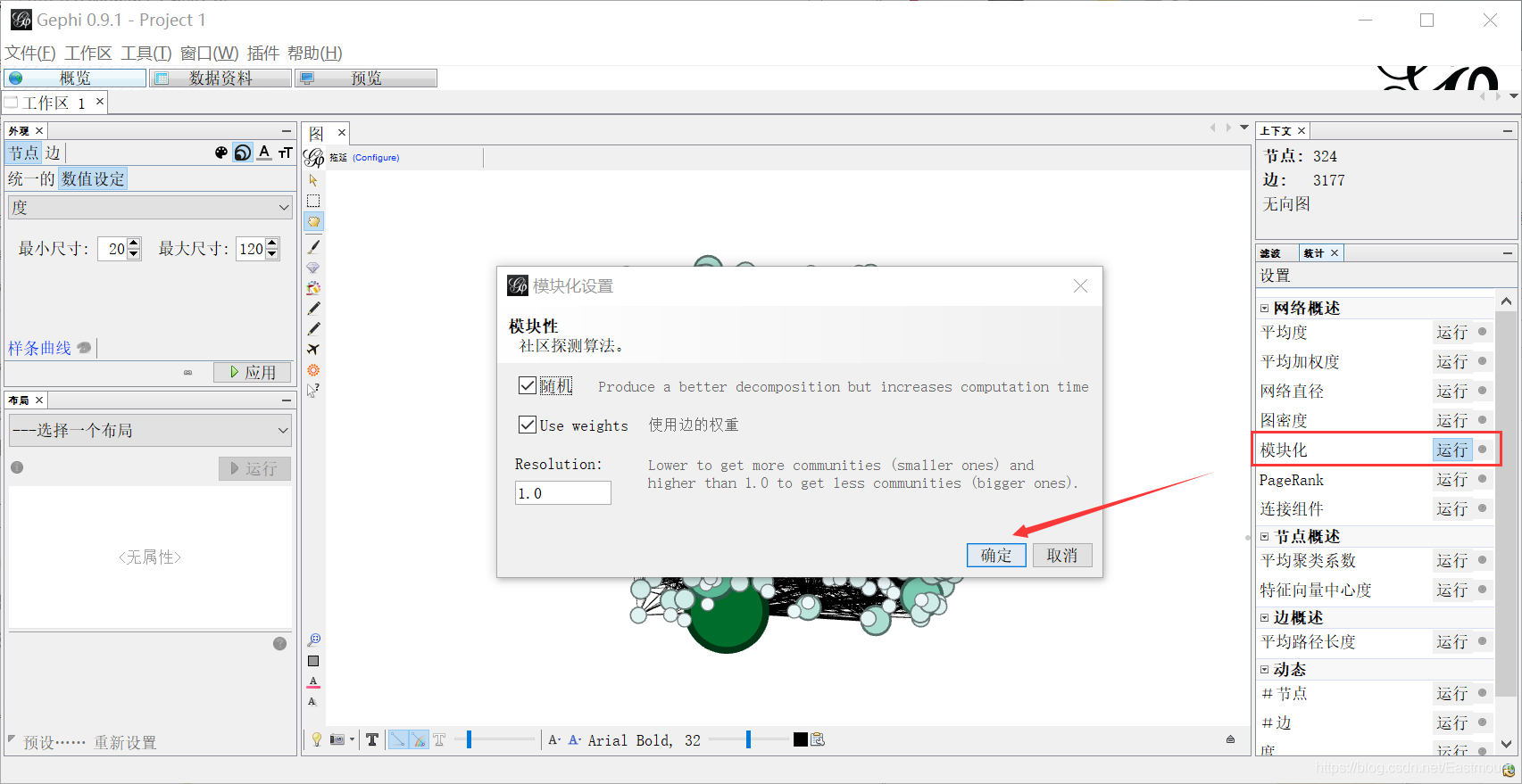
Step 6: set modularity. Click "run" in the statistics on the right to set modularity. At the same time, set the average path length. Click "run" in the statistics on the right to set the edge overview.

Step 7: reset the node attributes. The node size value is set to "degree". The minimum value is 20 and the maximum value is 120. The node color value is set to "Modularity Class", indicating modularity.
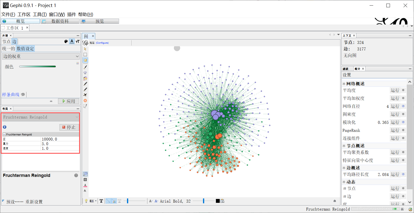
Step 8: select "Fruchterman Reingold" in the layout. Adjust area, gravity and speed.
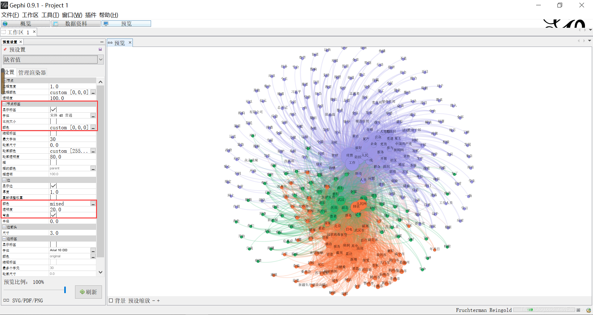
Step 9: click preview. Set the Song typeface, display the label, and adjust the transparency to 20, as shown in the figure below.
Step 10: map optimization and adjustment.
At the same time, you can filter the weight or set the light color of the color module. For example, get a more detailed relationship map.
7. Blog emotion analysis
SnowNLP experiment is mainly used for emotion analysis, and it is also recommended to use the emotion Dictionary of Dalian University of technology for optimization. Here are the articles previously analyzed by the author. The output results are shown in the figure below:
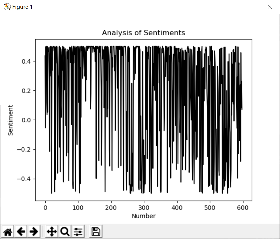
However, if we calculate the overall emotional score of daily or monthly news, we will reach the emotional analysis diagram of time series, so as to better predict the emotional trend. It is also widely used in the field of text mining or library and information.
# -*- coding: utf-8 -*-
from snownlp import SnowNLP
import codecs
import os

#Get emotional scores
source = open("06-data-fenci.txt", "r", encoding='gbk')
fw = open("09-result.txt", "w", encoding="gbk")
line = source.readlines()
sentimentslist = []
for i in line:
    s = SnowNLP(i)
    #print(s.sentiments)
    sentimentslist.append(s.sentiments)

#Interval conversion to [- 0.5, 0.5]
result = []
i = 0
while i<len(sentimentslist):
    result.append(sentimentslist[i]-0.5)
    fw.write(str(sentimentslist[i]-0.5)+"\n")
    print(sentimentslist[i]-0.5, line[i].strip("\n"))
    i = i + 1
fw.close()

#Visual drawing
import matplotlib.pyplot as plt
import numpy as np
plt.plot(np.arange(0, 598, 1), result, 'k-')
plt.xlabel('Number')
plt.ylabel('Sentiment')
plt.title('Analysis of Sentiments')
plt.show()
8. Analysis of blog theme evolution
The last is the subject of laboratory research. It is recommended that you read the core related papers of Nanjing University. In fact, theme evolution is usually divided into:
- Theme freshmen
- Theme extinction
- Theme fusion
- Theme loneliness
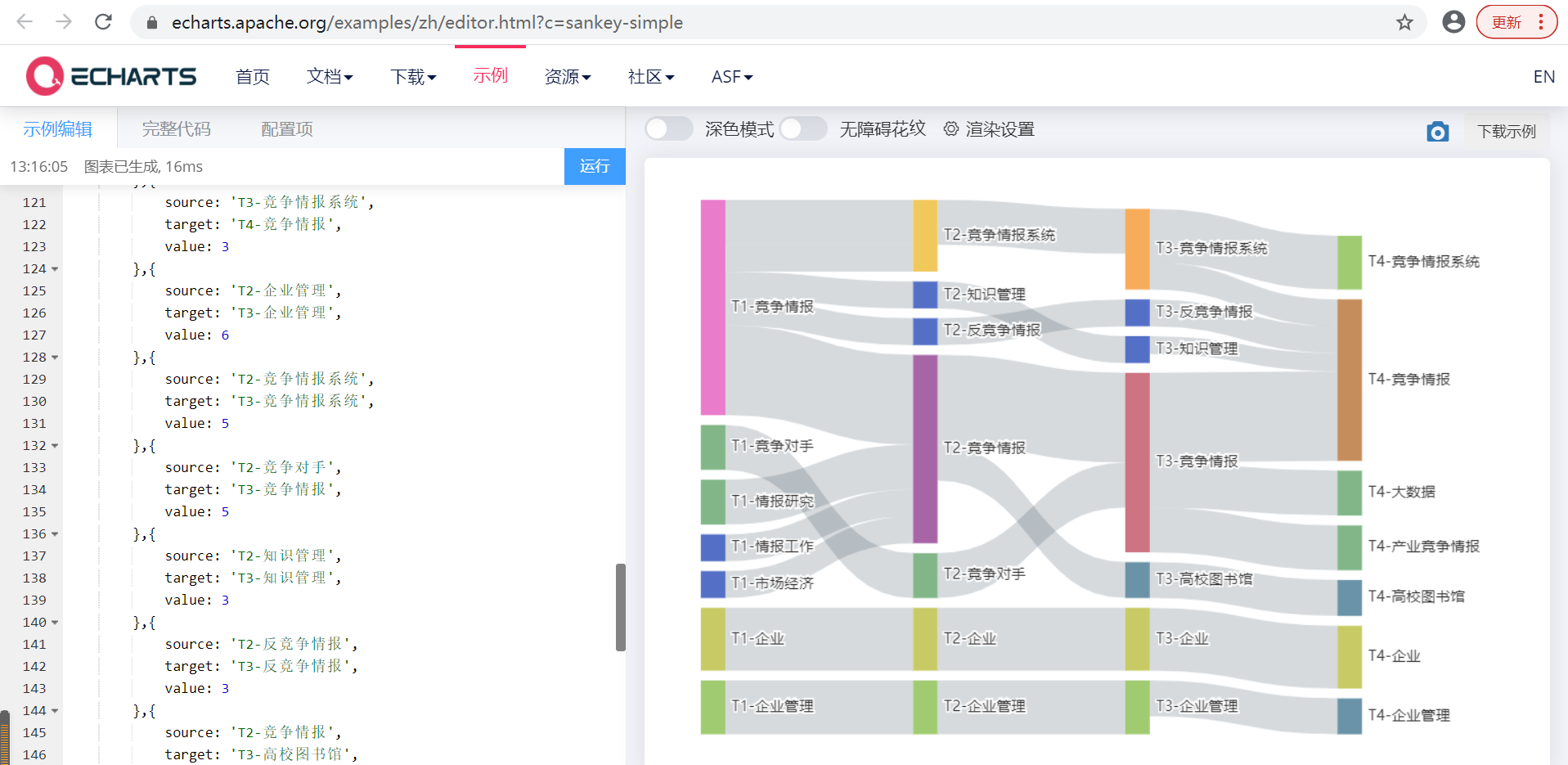
There are various calculation methods for topic fusion. You can find the most suitable method for your paper, such as word frequency, weight, O coefficient, relevance analysis and so on. It is recommended that you use Echarts to draw. The author's Atlas is shown in the figure below:
Note that the code given by the author here is another case. But the principle is the same, for reference only. The calculation process of the real situation is more complex, and the calculation evolution coefficient is usually decimal.
option = {
    series: {
        type: 'sankey',
        layout:'none',
        focusNodeAdjacency: 'allEdges',
        data: [
        {
            name: 'T1-competitive intelligence '
        },{
            name: 'T1-enterprise'
        },{
            name: 'T1-business management'
        }, {
            name: 'T1-Information research'
        },{
            name: 'T1-competitor'
        },{
            name: 'T1-Intelligence work'
        },{
            name: 'T1-market economy'
        },{
            name: 'T2-competitive intelligence '
        },{
            name: 'T2-enterprise'
        },{
            name: 'T2-business management'
        },{
            name: 'T2-Competitive intelligence system'
        },{
            name: 'T2-competitor'
        },{
            name: 'T2-knowledge management '
        },{
            name: 'T2-Anti competitive intelligence'
        },{
            name: 'T3-competitive intelligence '
        },{
            name: 'T3-enterprise'
        },{
            name: 'T3-Competitive intelligence system'
        },{
            name: 'T3-business management'
        },{
            name: 'T3-University Library'
        },{
            name: 'T3-Anti competitive intelligence'
        },{
            name: 'T3-knowledge management '
        },{
            name: 'T4-competitive intelligence '
        },{
            name: 'T4-enterprise'
        },{
            name: 'T4-big data'
        },{
            name: 'T4-Industrial Competitive Intelligence'
        },{
            name: 'T4-Competitive intelligence system'
        },{
            name: 'T4-University Library'
        },{
            name: 'T4-business management'
        }

        ],
        links: [{
            source: 'T1-competitive intelligence ',
            target: 'T2-competitive intelligence ',
            value: 10
        }, {
            source: 'T1-enterprise',
            target: 'T2-enterprise',
            value: 7
        }, {
            source: 'T1-business management',
            target: 'T2-business management',
            value: 6
        },{
            source: 'T1-Information research',
            target: 'T2-competitive intelligence ',
            value: 5
        },{
            source: 'T1-competitor',
            target: 'T2-competitor',
            value: 5
        },{
            source: 'T1-Intelligence work',
            target: 'T2-competitive intelligence ',
            value: 3
        },{
            source: 'T1-market economy',
            target: 'T2-competitive intelligence ',
            value: 3
        },{
            source: 'T1-competitive intelligence ',
            target: 'T2-Competitive intelligence system',
            value: 5
        },{
            source: 'T1-competitive intelligence ',
            target: 'T2-Competitive intelligence system',
            value: 3
        },{
            source: 'T1-competitive intelligence ',
            target: 'T2-knowledge management ',
            value: 3
        },{
            source: 'T1-competitive intelligence ',
            target: 'T2-Anti competitive intelligence',
            value: 3
        },

        {
            source: 'T2-competitive intelligence ',
            target: 'T3-competitive intelligence ',
            value: 10
        },{
            source: 'T2-enterprise',
            target: 'T3-enterprise',
            value: 7
        },{
            source: 'T3-Competitive intelligence system',
            target: 'T4-competitive intelligence ',
            value: 3
        },{
            source: 'T2-business management',
            target: 'T3-business management',
            value: 6
        },{
            source: 'T2-Competitive intelligence system',
            target: 'T3-Competitive intelligence system',
            value: 5
        },{
            source: 'T2-competitor',
            target: 'T3-competitive intelligence ',
            value: 5
        },{
            source: 'T2-knowledge management ',
            target: 'T3-knowledge management ',
            value: 3
        },{
            source: 'T2-Anti competitive intelligence',
            target: 'T3-Anti competitive intelligence',
            value: 3
        },{
            source: 'T2-competitive intelligence ',
            target: 'T3-University Library',
            value: 4
        },

        {
            source: 'T3-competitive intelligence ',
            target: 'T4-competitive intelligence ',
            value: 10
        },{
            source: 'T3-enterprise',
            target: 'T4-enterprise',
            value: 7
        },{
            source: 'T3-competitive intelligence ',
            target: 'T4-big data',
            value: 5
        },{
            source: 'T3-competitive intelligence ',
            target: 'T4-Industrial Competitive Intelligence',
            value: 5
        },{
            source: 'T3-Competitive intelligence system',
            target: 'T4-Competitive intelligence system',
            value: 6
        },{
            source: 'T3-business management',
            target: 'T4-business management',
            value: 4
        },
        {
            source: 'T3-University Library',
            target: 'T4-University Library',
            value: 4
        },{
            source: 'T3-Anti competitive intelligence',
            target: 'T4-competitive intelligence ',
            value: 3
        },{
            source: 'T3-knowledge management ',
            target: 'T4-competitive intelligence ',
            value: 2
        }

        ]
    }
};
The operation screenshot is as follows:
9. Expand knowledge
Readers can also carry out various text mining, such as:
- Named entity recognition
- Construction of knowledge map
- Intelligent question and answer processing
- Prediction of public opinion events
- ...
III summary
Finally, I sign my blog to end this article, "ignorance · optimism · low-key · humility · life". I always tell myself: ignorant, I need to be optimistic to seek knowledge. The background of low-key is humility, and humility comes from the insight into life. We not only have work, study and programming, but also learn to enjoy life. Why should we go in such a hurry and do some happy things in life, It's good to write a few systematic articles and bring a loved one! Thank CSDN for your persistence and sharing. This is more than ten years.
Thank all readers for their ten-year company, and disappear for a short time just to meet better. In the next three years, I am willing to accept my true self without inferiority or pride; I wish to work hard, live seriously, love what I love, have no regrets, and see you in the Jianghu. Welcome to leave a message and encourage each other~
(by: eastmount, 12:00 pm on April 28, 2021) http://blog.csdn.net/eastmount/ )