This learning note is the learning content of Alibaba cloud Tianchi Longzhu Docker training camp. The learning links are: https://tianchi.aliyun.com/notebook-ai/detail?spm=5176.20850282.J_3678908510.4.f2984d57AnIOhB&postId=170949

Task 2 purpose:
1. The value of EDA mainly lies in being familiar with the basic situation of the whole data set (missing value, abnormal value), verifying the data set, and whether the following machine learning or deep learning modeling can be carried out
2. Understand the relationship between variables and the existing relationship between variables and predicted values.
3. Preparation for characteristic Engineering

1. Summary of learning knowledge

• Learn how to analyze the overall overview of the data set, including the basic situation of the data set (missing values, outliers)
• Learn how to statistically organize data and filter by conditions
• Learn how to use matplotlib to visualize data

• Overall understanding of data
  • Read the data set and understand the size of the data set and the original feature dimension;
  • Familiar with data types through info;
  • Roughly view the basic statistics of each feature in the data set;
• Missing and unique values:
  • Check the missing data value
  • View unique value characteristics
• Drill down data - view data types
  • Category data
  • Numerical data
    • Discrete numerical data
    • Continuous numerical data
• Time format data processing and viewing
• Master PivotChart
• Using pandas_ Generating data report

2. Learning content

2.1 overall understanding of data

Import the library required for data analysis and visualization

import pandas as pd
import numpy as np
import matplotlib.pyplot as plt
import seaborn as sns
import datetime
import warnings
warnings.filterwarnings('ignore')
import pandas profiling

Read data

data_train = pd.read_csv('train.csv')
data_test_a = pd.read_csv('testA.csv')

If you encounter a table with too much data, you'd better add chunksize to read it in blocks
pd.read_csv usage

Check out what the data looks like

id	loanAmnt	term	interestRate	installment	   grade	subGrade	employmentTitle	employmentLength	homeOwnership	...	 n5	  n6    n7	   n8	  n9	 n10	 n11	n12    n13	 n14
0	35000.0	      5	        19.52	       917.97	     E	       E2	          320.0	         2 years	          2	        ...	9.0	  8.0	4.0	   12.0	  2.0	 7.0	 0.0	0.0	   0.0	 2.0

View data information
You can create an instance and substitute it into your own understanding, for example:
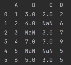
data_train=pd.DataFrame({"A":[1,2,3,4,5,6],"B":[3,4,NAN,7,NAN,5],"C":[2,NAN,3,7,NAN,3],"D":[2,6,7,9,5,5]})

data_train.info()#Overall data information
data_train.shape #Return the number of data rows and columns
data_train.columns #Return data column name
data_train.describe()#Returns some basic statistics of each feature of the data set, including mean, total number, maximum and minimum value, variance and major quantile
data_train.head(2).append(data_train.tail(2))#View the information of the first two columns and the last two columns, and connect them into a table with append

Specific column name introduction

• id is the unique L / C id assigned to the loan list
• loanAmnt loan amount
• Term loan term (year)
• interestRate loan interest rate
• installment amount
• Grade loan grade
• Sub grade of loan grade
• employmentTitle
• employmentLength of employment (years)
• homeOwnership the ownership status of the house provided by the borrower at the time of registration
• Annual income
• verificationStatus verification status
• issueDate month of loan issuance
• Purpose the loan purpose category of the borrower at the time of loan application
• postCode the first three digits of the postal code provided by the borrower in the loan application
• regionCode region code
• dti debt to income ratio
• delinquency_2years the number of default events in the borrower's credit file overdue for more than 30 days in the past two years
• ficoRangeLow is the lower limit range of fico of the borrower at the time of loan issuance
• ficoRangeHigh refers to the upper limit range of fico of the borrower at the time of loan issuance
• openAcc the number of open credit lines in the borrower's credit file
• pubRec detracts from the number of public records
• pubRecBankruptcies the number of public record purges
• Total revolving credit balance of revorbal
• revolUtil RCF utilization, or the amount of credit used by the borrower relative to all available RCFs
• totalAcc total current credit limit in the borrower's credit file
• Initial status list of loans
• applicationType indicates whether the loan is an individual application or a joint application with two co borrowers
• earliesCreditLine the month in which the borrower first reported the opening of the credit line
• title name of the loan provided by the borrower
• policyCode exposes available policies_ Code = 1 new product not publicly available policy_ Code = 2
• N-series anonymous features anonymous features n0-n14, which are the processing of some lender behavior counting features

2.2 missing and unique values

View features with missing values in feature attributes in training set and test set

print(len(data_train))#Returns the number of rows
print(data_train.isnull())##is.null() returns Boolean data in the corresponding data cell. If it is a missing value, it returns True. Otherwise, it returns False   
print(data_train.isnull().sum()) #sum() default column statistics sum parameters: 0-column, 1-row
print(data_train.isnull().any()) #any() returns True if it has one True. All() returns True only if it has all True
#any(0) column operation any(1) row operation
print(f'There are {data_train.isnull().any().sum()} columns in train dataset with missing values.') #Equivalent to print('There are {} columns in train dataset with missing values.'.format(data_train.isnull().any().sum()))#Here sum counts True

Run the above code to find that there are 22 columns of features with missing values in the training set. Then we can further check the features with a missing rate of more than 50% in the missing features

have_null_fea_dict = (data_train.isnull().sum()/len(data_train)).to_dict()#.to_dict() converts table data to dictionary format 
fea_null_moreThanHalf = {}
for key,value in have_null_fea_dict.items(): #Traversal dictionary
    if value > 0.5:
        fea_null_moreThanHalf[key] = value #Add a new element to the dictionary
print(fea_null_moreThanHalf)#Returns the desired feature

to_dict usage

matplotlib is used to visualize the data and check the missing characteristics and missing rate

missing = data_train.isnull().sum()/len(data_train) # Returns the missing rate. Missing is a series 
missing = missing[missing > 0] #Select data greater than 0 in missing
missing.sort_values(inplace=True )#sort_values is sorted by value size
missing.plot.bar()#Draw a bar chart

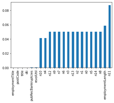
• Vertically understand which columns have "nan" and print the number of nan. The main purpose is to check whether the number of nan in a column is really large. If there are too many nan, it shows that this column has little effect on the label, so you can consider deleting it. If the missing value is very small, you can generally choose to fill.
• In addition, it can be compared horizontally. If most columns of some sample data are missing in the data set and there are enough samples, you can consider deleting * ***# data_train.dropna()

View features with only one value in the feature attribute in the training set and test set

#Unique returns the unique value and nunique returns the number of indicators
one_value_fea = [col for col in data_train.columns if data_train[col].nunique() <= 1] #Output result: ['policyCode ']
one_value_fea_test = [col for col in data_test_a.columns if data_test_a[col].nunique() <= 1] #Output result: ['policyCode ']

[col for col in data_train.columns if data_train[col].nunique()]
[return value iterator condition] returns a list
(n)unique usage

2.3 drill down data - view data types

• Features are generally composed of category features (object) and numerical features, and numerical features are divided into continuous and discrete.
• Category features sometimes have non numerical relationships and sometimes numerical relationships. For example, whether the grades A, B and C in 'grade' are just a simple classification or whether a is superior to others should be judged in combination with business.
• Numerical features can be directly put into the mold, but often the risk control personnel need to divide them into boxes, convert them into WOE codes, and then do standard score cards and other operations. From the perspective of model effect, feature box is mainly to reduce the complexity of variables, Reduce the influence of variable noise on the model , improve the correlation between independent variables and dependent variables. So as to make the model more stable.

View and filter data types

data_train.dtypes #The data types of each column can be returned. Note that as long as there is an object type, object will be returned
numerical_fea = list(data_train.select_dtypes(exclude=['object']).columns) #Select features based on data type
category_fea = list(filter(lambda x: x not in numerical_fea,list(data_train.columns)))
#The filter() function is used to filter the sequence. It will filter out the unqualified data. The result returned by the filter function is an iterative object.
#If the second code does not start with a list, you need to iterate through the for loop

filter function usage

Filtering numerical type category features: it is divided into columns with the number of results greater than 10 and ≤ 10. In fact, it is also an operation to divide variables into continuous and discrete types, which is convenient for statistics and bar statistics of discrete data, and line chart or kernel density square chart of continuous data

def get_numerical_serial_fea(data,feas):
    numerical_serial_fea = []
    numerical_noserial_fea = []
    for fea in feas:
        temp = data[fea].nunique()#Filter condition
        if temp <= 10:
            numerical_noserial_fea.append(fea)
            continue
        numerical_serial_fea.append(fea)
    return numerical_serial_fea,numerical_noserial_fea
numerical_serial_fea,numerical_noserial_fea = get_numerical_serial_fea(data_train,numerical_fea)

#The returned discrete variables are:
numerical_noserial_fea: ['term','homeOwnership','verificationStatus','isDefault','initialListStatus','applicationType','policyCode','n11','n12']

Statistics of discrete variables value_count()

data_train['term'].value_counts()

3    606902
5    193098
Name: term, dtype: int64
-------------------------------
data_train['homeOwnership'].value_counts()

0    395732
1    317660
2     86309
3       185
5        81
4        33
Name: homeOwnership, dtype: int64

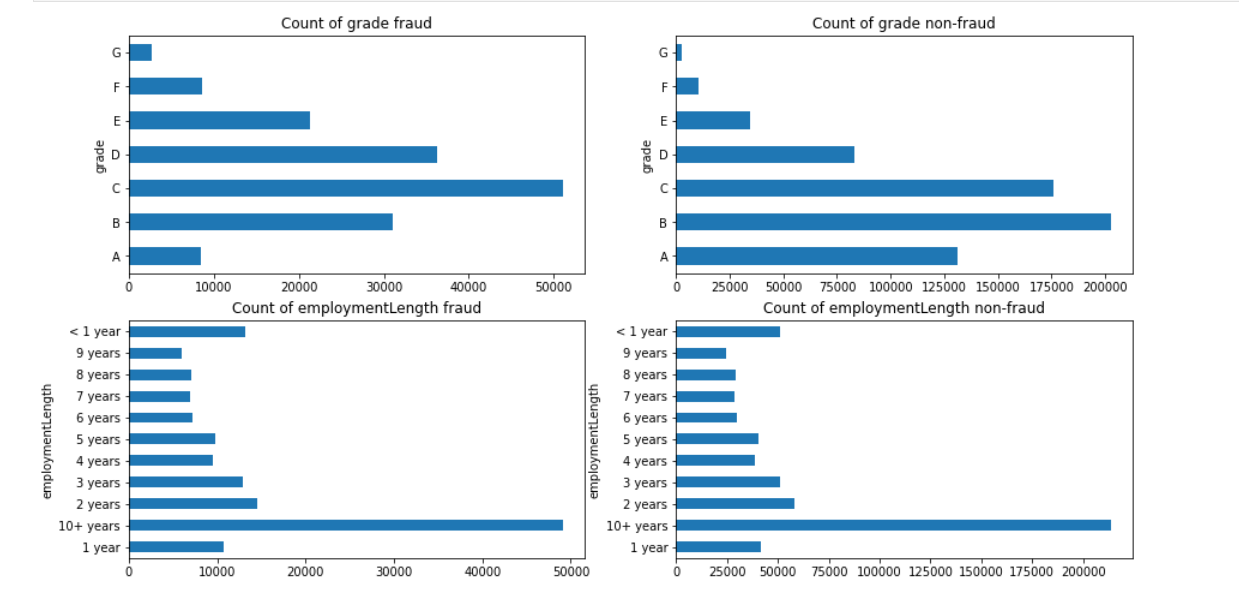
Visualize the distribution of a feature of x according to different y values

• First, check the distribution of category variables on different y values
• Then visual analysis is carried out according to the distribution

train_loan_fr = data_train.loc[data_train['isDefault'] == 1] #The loc function selects data. Another is iloc. You can check reindex again
train_loan_nofr = data_train.loc[data_train['isDefault'] == 0]
fig, axes = plt.subplots(2, 2, figsize=(15, 8))
train_loan_fr.groupby('grade')['grade'].count().plot(kind='barh', ax=axes[0,0], title='Count of grade fraud')
train_loan_nofr.groupby('grade')['grade'].count().plot(kind='barh', ax=axes[0,1], title='Count of grade non-fraud')
train_loan_fr.groupby('employmentLength')['employmentLength'].count().plot(kind='barh', ax=axes[1,0], title='Count of employmentLength fraud')
train_loan_nofr.groupby('employmentLength')['employmentLength'].count().plot(kind='barh', ax=axes[1,1], title='Count of employmentLength non-fraud')
plt.show()

Usage of loc and iloc functions

Visual distribution of continuous variables

f = pd.melt(data_train, value_vars=numerical_serial_fea) #pd.melt changes the wide perspective to long, PD Pivot changes long perspective to wide perspective
g = sns.FacetGrid(f, col="variable",  col_wrap=2, sharex=False, sharey=False) #col_wrap=2, two subgraphs per line
g = g.map(sns.distplot, "value")#Square nucleation density map https://www.sogou.com/link?url=hedJjaC291P3yGwc7N55kLSc2ls_Ks2xmk1vI0c0xdDbaJ2KBnWAiC--N4hJvhoHri2jTBr9OJ8.

FaceGrid usage
Usage of the plot function

Screenshot of some charts

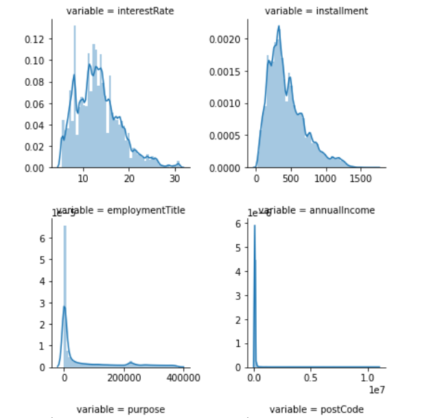
• If the distribution of a variable does not conform to the normal distribution of wilpiu#, you can check whether the value of the next variable does not conform to the normal distribution of wilpiu#.
• If you want to deal with a batch of data uniformly and become standardized, you must put forward these previously normalized data
• Reasons for normalization: in some cases, normal and non normal can make the model converge faster. Some models require data normality (eg. GMM, KNN) to ensure that the data is not too skewed, which may affect the prediction results of the model.

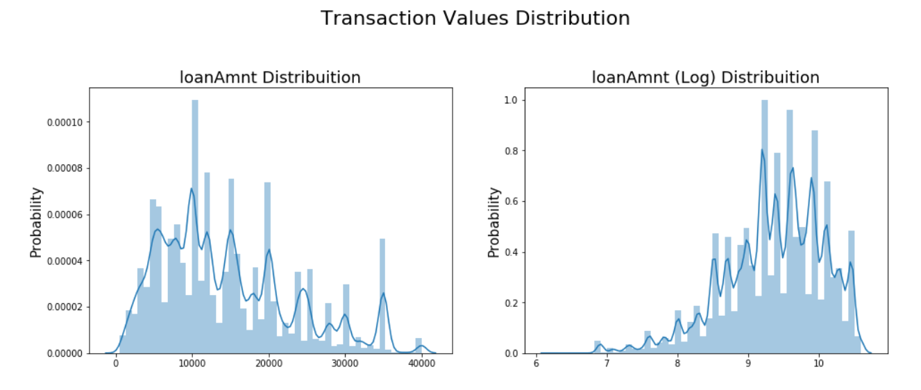
Compare the distribution of original data and log data

plt.figure(figsize=(16,8))
plt.suptitle('Transaction Values Distribution', fontsize=22)#Add general title
plt.subplot(121)#Draw the first subgraph. The subgraphs are arranged as 2 × The position of matrix subplot(121) of 2 is equivalent to the position of (1,1)
sub_plot_1 = sns.distplot(data_train['loanAmnt'])
sub_plot_1.set_title("loanAmnt Distribuition", fontsize=18) #Set icon title
sub_plot_1.set_xlabel("") #Set x-axis label
sub_plot_1.set_ylabel("Probability", fontsize=15) #Set y-axis label

plt.subplot(122)
sub_plot_2 = sns.distplot(np.log(data_train['loanAmnt']))
sub_plot_2.set_title("loanAmnt (Log) Distribuition", fontsize=18)
sub_plot_2.set_xlabel("") 
sub_plot_2.set_ylabel("Probability", fontsize=15)

2.4 time format data processing and viewing

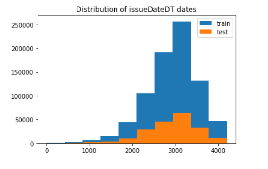
#The issueDateDT feature converted to time format indicates the number of days from the date of the data date to the earliest date in the dataset (2007-06-01)
data_train['issueDate'] = pd.to_datetime(data_train['issueDate'],format='%Y-%m-%d')
startdate = datetime.datetime.strptime('2007-06-01', '%Y-%m-%d')#Convert string to date strftime: format the date into a string
data_train['issueDateDT'] = data_train['issueDate'].apply(lambda x: x-startdate).dt.days 

to_datetime and DT days

Some knowledge of time series can be viewed in the file resources I uploaded, which is the notes I made when I studied "data analysis using python"

#Convert to time format
data_test_a['issueDate'] = pd.to_datetime(data_train['issueDate'],format='%Y-%m-%d')
startdate = datetime.datetime.strptime('2007-06-01', '%Y-%m-%d')
data_test_a['issueDateDT'] = data_test_a['issueDate'].apply(lambda x: x-startdate).dt.days

plt.hist(data_train['issueDateDT'], label='train');
plt.hist(data_test_a['issueDateDT'], label='test');
plt.legend();
plt.title('Distribution of issueDateDT dates');
#train and test issueDateDT dates overlap, so it is unwise to use time-based segmentation for verification

2.5 master PivotChart

Using pandas_ Generating data report

print(tips[:5])
print(tips.pivot_table(['total_bill'],index=['time','smoker'],columns='day',margins=True,aggfunc='mean',fill_value=0))
#The first parameter is the operation target. index means to select row indicators, columns means to select column indicators, margins means to add row and column totals, which is ALL in the figure, aggfunc means to perform function operations, and fill_value=0 means to replace the missing value in the figure with 0

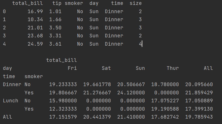
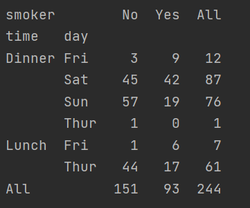
Expand the cross tab cross table

print(pd.crosstab([tips.time,tips.day],tips.smoker,margins=True)) #The first two parameters are rows and columns

2.6 using pandas_ Generating data report

import pandas_profiling
pfr = pandas_profiling.ProfileReport(data_train)
pfr.to_file("./example.html")

Because I don't know the above reasons, I can't generate the report. Post an article from other coders below
python automatic data analysis -- pandas_profiling

3, Learning questions and answers

The thinking and solution of the code has been integrated into the second point

4, Learning, thinking and summary

Data exploratory analysis is the stage when we initially understand the data, get familiar with the data and prepare for Feature Engineering. Even many times, the features extracted in EDA stage can be directly used as rules. We can see the importance of EDA. The main work at this stage is to understand the overall data with the help of various simple statistics, analyze the relationship between various types of variables, and visualize them with appropriate graphics