1. Overview of Research Report
This article is the second in the recurrence series of the securities company metalworking Research Report. The text reproduces the market timing based on the relative strength of resistance support (RSRS) of Everbright Securities.
The traditional application method of resistance level and support level is to select specific resistance level and support level as the threshold to build breakthrough and reversal strategies. Common strategies such as moving average strategy: [if the closing price of the day exceeds the 20 day moving average, build a position and buy. Hold the position until the closing price is lower than the 20 day moving average, sell and close the position].
Different from the traditional application method of selecting the threshold interval of resistance level and support level, this research report focuses on the relative strength of resistance level and support level.
The resistance level and support level actually reflect the traders' expected judgment on the top and bottom of the market state.
Intuitively, if this expectation judgment is easy to change, it indicates that the strength of support level or resistance level is small and the effectiveness is weak; If the expectations of many traders are relatively consistent and change little, it indicates that the strength of support level or resistance level is high and the effectiveness is strong.
If the strength of the support level is small and the effect is weaker than the resistance level, it indicates that the market participants have more differences on the support level than on the resistance level, and the market is more inclined to change to a bear market next. If the strength of the support level is strong and the effect is stronger than the resistance level, it means that the market participants' recognition of the support level is higher than that of the resistance level, and the market tends to change in the bull market.
We illustrate the application logic of the relative strength of support resistance according to different market conditions:
1. The market is in a rising bull market:
If support is significantly stronger than resistance, the bull market will continue and prices will accelerate
If the resistance is significantly stronger than the support, the bull market may be coming to an end and the price will peak
2. The market is in shock:
If support is significantly stronger than resistance, the bull market may be about to start
If resistance is significantly stronger than support, a bear market may be about to start
3. The market is in a downward bear market:
If the support is obviously stronger than the resistance, the bear market may be coming to an end and the price bottoms out
If the resistance is obviously stronger than the support, the bear market will continue and the price will fall faster
This research report constructs an index RSRS (Resistance Support Relative Strength) to measure the relative strength between resistance level and support level. When the strength of support level is small and the strength of resistance level is large, the value of RSRS is high, on the contrary, the value of RSRS is low.
2. Research environment
Data source: jukuan JoinQuant, daily data from June 2005 to may 2017
import datetime
import math
import numpy as np
import matplotlib.pyplot as plt
import pandas as pd
import statsmodels.api as sm
import warnings
warnings.filterwarnings("ignore")
plt.rcParams['font.sans-serif'] = ['SimHei']
plt.rcParams['axes.unicode_minus'] = False
3. Reproduction of Research Report
3.1 quantifying the relative strength of resistance level and support level RSRS
The primary problem to be solved in the research report is how to define and quantify the relative strength of resistance level and support level, and to solve this problem, we must first select a pair of appropriate resistance level and support level indicators.
3.1.1 how to select resistance level and support level
The first step to quantify the relative strength between resistance level and support level is to select appropriate resistance level and support level indicators. In the school of technical analysis, there have been many definitions of support level and resistance level, including channel line (upper and lower rails of brin belt), front high and front low in a period of time, Interval Oscillation line (DPO), etc.
The Research Report selects the daily highest price and lowest price as the resistance level and support level, because the daily highest price and lowest price can quickly reflect the nature of the recent market attitude towards resistance level and support level.
3.1.2 basic idea of RSRS construction
This research report puts forward a variety of quantitative methods of relative strength, and the relationship is optimized layer by layer.
Here is a brief introduction to each method, and the effect of the strategy constructed by each quantitative method will be given later.
Basic idea:
Here, the relative change rates of the highest price and the lowest price are used, that is, values similar to delta (high) / delta (low)
The relative strength of the support level and the resistance level, that is, the change range of the highest price when the lowest price changes by 1.
Based on this basic idea, the original research report uses
Slope of linear regression line
Slope standard score
Revised standard score
Right standard score
Four methods are used to quantify the relative strength of resistance support. These four methods are progressive and optimized layer by layer.
Finally, combined with the price and volume data optimization strategy. This paper will give the calculation method and the effect of the construction strategy for each method.
3.2 specific calculation method and strategy effect
3.2.0 data format and strategy statistical function
Before giving the specific policy code, we first introduce the data format used by the policy.
In the policy backtesting, we use DataFrame format data df. It includes not only the time series of price and RSRS indicators, but also flag and position.
Flag is the opening and closing flag bit. When df ['flag'] [i] is 1, it indicates that the opening operation is carried out on the I day, and when df ['flag'] [i] is - 1, it indicates that the closing operation is carried out on the I day. Position is the position flag of the account. A value of 1 indicates that the current account holds securities, and a value of 0 indicates that the current account is empty.
At the same time, in the strategy constructed in this paper, the buying operation is only carried out when the current account is empty.
Here, we first give the function of statistical strategy results, which will be used many times later.
def calculate_statistics(df):
    '''
    Input:
    DataFrame Type, including price data, position and opening / closing flag
        position Column: position flag, 0 indicates empty position, 1 indicates holding target
        flag Column: buy sell flag, 1 means buy at this time,-1 Means to sell at that time
        close Column: daily closing price

    Output: dict Type, including statistical data of strategy results such as sharp ratio and maximum pullback
    '''
    #Net worth series
    df['net_asset_pct_chg'] = df.net_asset_value.pct_change(1).fillna(0)

    #Total rate of return and annualized rate of return
    total_return = (df['net_asset_value'][df.shape[0]-1] -1)
    annual_return = (total_return)**(1/(df.shape[0]/252)) -1
    total_return = total_return*100
    annual_return = annual_return*100
    #sharpe ratio
    df['ex_pct_chg'] = df['net_asset_pct_chg']
    sharp_ratio = df['ex_pct_chg'].mean() * math.sqrt(252)/df['ex_pct_chg'].std()

    #retracement
    df['high_level'] = (
            df['net_asset_value'].rolling(
            min_periods=1, window=len(df), center=False).max()
    )
    df['draw_down'] = df['net_asset_value'] - df['high_level']
    df['draw_down_percent'] = df["draw_down"] / df["high_level"] * 100
    max_draw_down = df["draw_down"].min()
    max_draw_percent = df["draw_down_percent"].min()

    #Total days of positions
    hold_days = df['position'].sum()

    #Number of transactions
    trade_count = df[df['flag']!=0].shape[0]/2

    #Average position days
    avg_hold_days = int(hold_days/trade_count)

    #Profit days
    profit_days = df[df['net_asset_pct_chg'] > 0].shape[0]
    #Loss days
    loss_days = df[df['net_asset_pct_chg'] < 0].shape[0]

    #Winning rate (by day)
    winrate_by_day = profit_days/(profit_days+loss_days)*100
    #Average profit rate (by day)
    avg_profit_rate_day = df[df['net_asset_pct_chg'] > 0]['net_asset_pct_chg'].mean()*100
    #Average loss rate (by day)
    avg_loss_rate_day = df[df['net_asset_pct_chg'] < 0]['net_asset_pct_chg'].mean()*100
    #Average profit loss ratio (by day)
    avg_profit_loss_ratio_day = avg_profit_rate_day/abs(avg_loss_rate_day)


    #Each transaction
    buy_trades = df[df['flag']==1].reset_index()
    sell_trades = df[df['flag']==-1].reset_index()
    result_by_trade = {
        'buy':buy_trades['close'],
        'sell':sell_trades['close'],
        'pct_chg':(sell_trades['close']-buy_trades['close'])/buy_trades['close']
    }
    result_by_trade = pd.DataFrame(result_by_trade)
    #Profit times
    profit_trades = result_by_trade[result_by_trade['pct_chg']>0].shape[0]
    #Number of losses
    loss_trades = result_by_trade[result_by_trade['pct_chg']<0].shape[0]
    #Single maximum profit
    max_profit_trade = result_by_trade['pct_chg'].max()*100
    #Single maximum loss
    max_loss_trade = result_by_trade['pct_chg'].min()*100
    #Winning rate (by times)
    winrate_by_trade = profit_trades/(profit_trades+loss_trades)*100
    #Average profit rate (by time)
    avg_profit_rate_trade = result_by_trade[result_by_trade['pct_chg'] > 0]['pct_chg'].mean()*100
    #Average loss rate (by time)
    avg_loss_rate_trade = result_by_trade[result_by_trade['pct_chg'] < 0]['pct_chg'].mean()*100
    #Average profit loss ratio (by times)
    avg_profit_loss_ratio_trade = avg_profit_rate_trade/abs(avg_loss_rate_trade)

    statistics_result = {
        'net_asset_value':df['net_asset_value'][df.shape[0]-1],#Final net worth
        'total_return':total_return,#Yield
        'annual_return':annual_return,#Annualized rate of return
        'sharp_ratio':sharp_ratio,#sharpe ratio
        'max_draw_percent':max_draw_percent,#Maximum pullback
        'hold_days':hold_days,#Position days
        'trade_count':trade_count,#Number of transactions
        'avg_hold_days':avg_hold_days,#Average position days
        'profit_days':profit_days,#Profit days
        'loss_days':loss_days,#Loss days
        'winrate_by_day':winrate_by_day,#Winning rate (by day)
        'avg_profit_rate_day':avg_profit_rate_day,#Average profit rate (by day)
        'avg_loss_rate_day':avg_loss_rate_day,#Average loss rate (by day)
        'avg_profit_loss_ratio_day':avg_profit_loss_ratio_day,#Average profit loss ratio (by day)
        'profit_trades':profit_trades,#Profit times
        'loss_trades':loss_trades,#Number of losses
        'max_profit_trade':max_profit_trade,#Single maximum profit
        'max_loss_trade':max_loss_trade,#Single maximum loss
        'winrate_by_trade':winrate_by_trade,#Winning rate (by times)
        'avg_profit_rate_trade':avg_profit_rate_trade,#Average profit rate (by time)
        'avg_loss_rate_trade':avg_loss_rate_trade,#Average loss rate (by time)
        'avg_profit_loss_ratio_trade':avg_profit_loss_ratio_trade#Average profit loss ratio (by times)
    }
    return statistics_result
3.2.1 slope method
Because there is noise in the market, it is considered to use the slope of the linear regression model of the highest and lowest prices for N consecutive days to quantify the relative strength of support level and resistance level, so as to increase the signal-to-noise ratio.
That is, take the linear regression model of the highest price and the lowest price for N consecutive days
high = alpha + beta*low
The beta in, that is, the slope of the line, is used as our relative strength RSRS.
Calculation method of slope index:
- Take the highest price sequence and the lowest price sequence of the previous N days.
- Perform OLS linear regression on the two columns of data according to the model of formula (1).
- Take the fitted beta value as the RSRS slope index value of the current day.
In the original research report, through the comparison of different values of N, when n is 18, the quantitative index construction strategy is more effective.
Based on the slope method, the construction strategy:
- Calculate the RSRS slope.
- If the hold slope is greater than 1, then hold.
- If the slope is less than 0.8, the seller will close the position.
Policy source code
#Calculation method of current day slope index, linear regression
def cal_nbeta(df,n):
    nbeta = []
    trade_days = len(df.index)

    df['position'] = 0
    df['flag'] = 0
    position = 0

  #Calculate slope value
    for i in range(trade_days):
        if i < (n-1):
            #In order to match n-1, the iloc index is used next
            continue
        else:
            x = df['low'].iloc[i-n+1:i+1]
            #iloc left closed right open
            x = sm.add_constant(x)
            y = df['high'].iloc[i-n+1:i+1]
            regr = sm.OLS(y,x)
            res = regr.fit()
            beta = round(res.params[1],2)#Slope index
            nbeta.append(beta)
    df1 = df.iloc[n-1:]
    df1['beta'] = nbeta

  #Execute trading strategy
    for i in range(len(df1.index)-1):
        #Here - 1 is to avoid the last line
        if df1['beta'].iloc[i] > 1 and position == 0:
            df1['flag'].iloc[i] = 1 #Opening sign
            df1['position'].iloc[i+1] =1 #Bin is not empty
            position = 1
        elif df1['beta'].iloc[i] < 0.8 and position == 1:
            df1['flag'].iloc[i] = -1 #Closing mark
            df1['position'].iloc[i+1] = 0 #Empty bin
            position = 0
        else:
            df1['position'].iloc[i+1] = df1['position'].iloc[i]
    #Calculate net worth series
    df1['net_asset_value'] = (1+df1.close.pct_change(1).fillna(0)*df1.position).cumprod()
    return df1
Strategic net worth curve
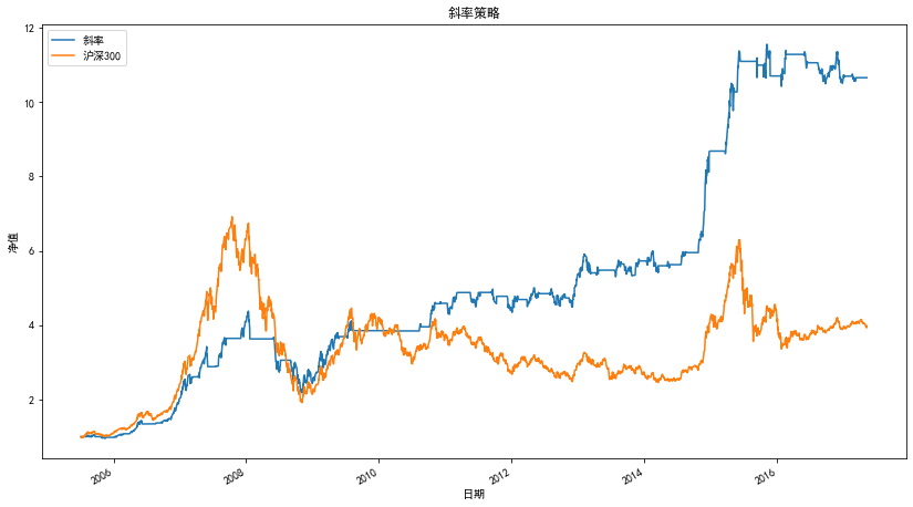
Statistical indicators of strategy
| statistic | Slope strategy |
|---|---|
| net worth | 10.66 |
| Yield | 965.73% |
| Annualized rate of return | 21.92% |
| sharpe ratio | 1.16 |
| Maximum pullback | -50.26% |
| Position days | 1184 |
| Number of transactions | 21 |
| Average position days | 56 |
| Profit days | 747 |
| Loss days | 575 |
| Winning rate (by day) | 56.51% |
| Average profit rate (by day) | 1.31% |
| Average loss rate (by day) | -1.25% |
| Average profit loss ratio (by day) | 1.05 |
| Profit times | 16 |
| Number of losses | 5 |
| Single maximum profit | 170% |
| Single maximum loss | -12% |
| Winning rate (by times) | 76.19% |
| Average profit rate (by time) | 25% |
| Average loss rate (by time) | -3% |
| Average profit loss ratio (by times) | 7.86 |
3.2.2 optimization of slope method - slope standard score
When using the slope index to construct the strategy, we need to refer to the historical mean and standard deviation of the slope index to select the appropriate opening and closing threshold.
However, as the market changes at any time, the mean and standard deviation of data in different periods may change. At the same time, traders may also be more concerned about the position of the current market in the recent environment, or how the market will develop in the next period of time. Therefore, compared with directly using the mean and standard deviation of the slope in the whole history to help select the threshold, determining the threshold according to the standard score of the slope in the recent certain cycle (600 trading days) can more flexibly adapt to the recent basic state of the overall market.
Calculation method of slope standard score:
- Take the slope time series of the previous M days.
- Calculate the standard score of the slope of the day based on this sample.
- Take the calculated standard score z as the RSRS standard score index value of the current day.
Build standard sub strategy:
1. Calculate the standard score according to the slope (parameter N=18,M=600).
2. If the standard score is greater than S (parameter S=0.7), buy and hold.
3. If the standard score is less than - S, sell and close the position.
Policy source code
#Standard sub strategy
def cal_stdbeta(df,n):

    df['position'] = 0
    df['flag'] = 0
    position = 0

    df1 = cal_nbeta(df,n)
    pre_stdbeta = df1['beta']
    pre_stdbeta = np.array(pre_stdbeta)
    #Into an array, you can operate on the entire array
    sigma = np.std(pre_stdbeta)
    mu = np.mean(pre_stdbeta)
    #Standardization
    stdbeta = (pre_stdbeta-mu)/sigma

    df1['stdbeta'] = stdbeta

    for i in range(len(df1.index)-1):
        #Here - 1 is to avoid the last line
        if df1['stdbeta'].iloc[i] > 0.7 and position == 0:
            df1['flag'].iloc[i] = 1
            df1['position'].iloc[i+1] =1
            position = 1
        elif df1['stdbeta'].iloc[i] < -0.7 and position == 1:
            df1['flag'].iloc[i] = -1
            df1['position'].iloc[i+1] = 0
            position = 0
        else:
            df1['position'].iloc[i+1] = df1['position'].iloc[i]

    df1['net_asset_value'] = (1+df1.close.pct_change(1).fillna(0)*df1.position).cumprod()
    return df1
#stdbeta is an array and beta is a list
Net worth curve
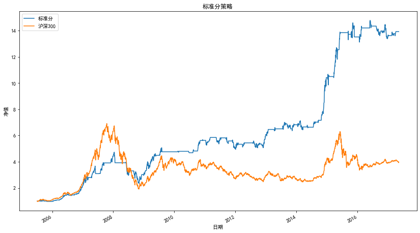
Statistical indicators of strategy
| statistic | Standard sub strategy |
|---|---|
| net worth | 13.93 |
| Yield | 1292.70% |
| Annualized rate of return | 25.07% |
| sharpe ratio | 1.28 |
| Maximum pullback | -50.26% |
| Position days | 1298 |
| Number of transactions | 67 |
| Average position days | 19 |
| Profit days | 741 |
| Loss days | 557 |
| Winning rate (by day) | 57.09% |
| Average profit rate (by day) | 1.32% |
| Average loss rate (by day) | -1.25% |
| Average profit loss ratio (by day) | 1.06 |
| Profit times | 40 |
| Number of losses | 26 |
| Single maximum profit | 91% |
| Single maximum loss | -41% |
| Winning rate (by times) | 60.61% |
| Average profit rate (by time) | 18% |
| Average loss rate (by time) | -9% |
| Average profit loss ratio (by times) | 2.05 |
3.2.3 re optimization - modify the standard score: consider the degree of linear fitting
When linear regression is used to fit the slope of the straight line or its standard score as the relative strength, the absolute value of the slope or standard score may be very large, but the fitting effect of the straight line itself is not good, so that the slope or the standard score of the slope itself can not well reflect the relative strength. When the relative strength index needs to be constructed, the quality of the fitting result of the linear model can be considered.
In linear regression, the square value of R (determination coefficient) can be understood as the degree of linear fitting effect.
Therefore, use
Corrected standard score = standard score * R square value (determination coefficient)
To quantify the relative strength can weaken the influence of straight-line fitting effect on the index effect.
Construct and revise standard sub strategy
- Calculate the corrected standard score (N=16,M=300).
- If the corrected standard score is greater than S (S=0.7), buy and hold.
- If the corrected standard score is less than - S, sell and close the position.
Policy source code
#Optimization of RSRS standard sub index and correction of standard sub index
def cal_better_stdbeta(df,n):
    nbeta = []
    R2 = []
    trade_days = len(df.index)
    for i in range(trade_days):
        if i < (n-1):
            #In order to match n-1, the iloc index is used next
            continue
        else:

            x = df['low'].iloc[i-n+1:i+1]
            #iloc left closed right open
            x = sm.add_constant(x)
            y = df['high'].iloc[i-n+1:i+1]
            regr = sm.OLS(y,x)
            res = regr.fit()
            beta = round(res.params[1],2)

            R2.append(res.rsquared)
            nbeta.append(beta)

    prebeta = np.array(nbeta)
    sigma = np.std(prebeta)
    mu = np.mean(prebeta)
    stdbeta = (prebeta-mu)/sigma

    r2 = np.array(R2)
    better_stdbeta = r2*stdbeta#Revised standard score

    df1 = df.iloc[n-1:]
    df1['beta'] = nbeta
    df1['flag'] = 0
    df1['position'] = 0
    position = 0
    df1['better_stdbeta'] = better_stdbeta

    for i in range(len(df1.index)-1):
        #Here - 1 is to avoid the last line
        if df1['better_stdbeta'].iloc[i] > 0.7 and position == 0:
            df1['flag'].iloc[i] = 1
            df1['position'].iloc[i+1] =1
            position = 1
        elif df1['better_stdbeta'].iloc[i] < -0.7 and position == 1:
            df1['flag'].iloc[i] = -1
            df1['position'].iloc[i+1] = 0
            position = 0
        else:
            df1['position'].iloc[i+1] = df1['position'].iloc[i]
    df1['net_asset_value'] = (1+df1.close.pct_change(1).fillna(0)*df1.position).cumprod()
    return df1
Strategic net worth curve
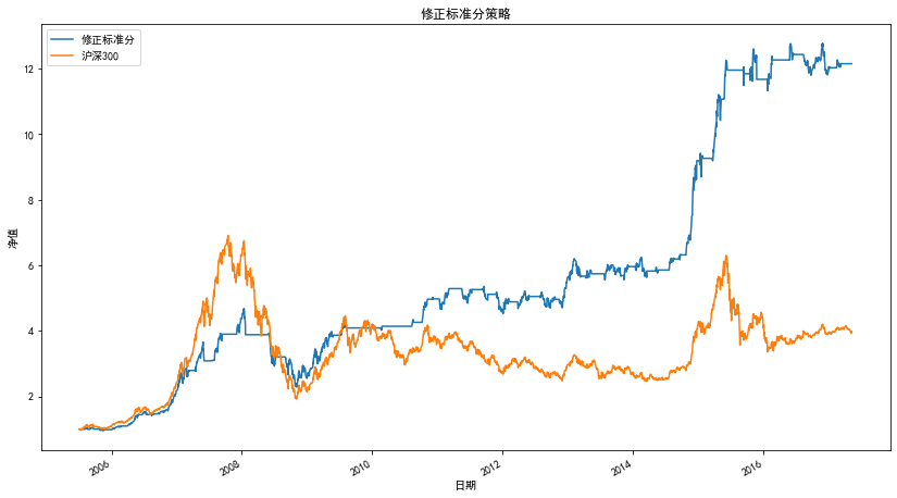
Strategic indicators
| amount | Revised standard sub strategy |
|---|---|
| net worth | 12.15 |
| Yield | 1115.40% |
| Annualized rate of return | 23.47% |
| sharpe ratio | 1.19 |
| Maximum pullback | -51.28% |
| Position days | 1397 |
| Number of transactions | 46 |
| Average position days | 30 |
| Profit days | 790 |
| Loss days | 607 |
| Winning rate (by day) | 56.55% |
| Average profit rate (by day) | 1.30% |
| Average loss rate (by day) | -1.25% |
| Average profit loss ratio (by day) | 1.05 |
| Profit times | 32 |
| Number of losses | 14 |
| Single maximum profit | 76% |
| Single maximum loss | -18% |
| Winning rate (by times) | 69.57% |
| Average profit rate (by time) | 11% |
| Average loss rate (by time) | -3% |
| Average profit loss ratio (by times) | 3.3 |
3.2.4 re optimization - right standard score: conjecture in the process of practice
When analyzing and comparing the correlation between the standard score and the revised standard score on the future market, the original research report found that the standard score on the right (i.e. z > 0) has good predictability on the future market income, while the standard score on the left has lost predictability. Because the standard score on the left accounts for most of the whole, the correlation between the overall standard score and the future market income is low. The value range on the right side of the revised standard score is expanded (not an absolute value range compared with the left side), and the revised standard score shows better predictability as a whole.
Therefore, guess: is the wider the value range on the right (not an absolute value range compared to the left), the better the predictability of the index?
In order to verify the conjecture, the right standard score is constructed
Right standard score = corrected standard score * slope
Constructing right deviation standard score strategy
- Calculate the right deviation standard score (N=16,M=300).
- If the right standard score is greater than S (S=0.7), buy and hold.
- If the right standard score is less than - S, sell and close the position.
Policy source code
#The standard score of right deviation is 16 at this time
def cal_right_stdbeta(df,n):

    df1 = cal_better_stdbeta(df,n)
    df1['position'] = 0
    df1['flag'] = 0
    df1['net_value'] = 0
    position = 0

    df1['right_stdbeta'] = df1['better_stdbeta']*df1['beta']
    #The modified standard score multiplied by the slope value can make the original distribution to the right

    for i in range(len(df1.index)-1):
        #Here - 1 is to avoid the last line
        if df1['right_stdbeta'].iloc[i] > 0.7 and position == 0:
            df1['flag'].iloc[i] = 1
            df1['position'].iloc[i+1] =1
            position = 1
        elif df1['right_stdbeta'].iloc[i] < -0.7 and position == 1:
            df1['flag'].iloc[i] = -1
            df1['position'].iloc[i+1] = 0
            position = 0
        else:
            df1['position'].iloc[i+1] = df1['position'].iloc[i]
    df1['net_asset_value'] = (1+df1.close.pct_change(1).fillna(0)*df1.position).cumprod()
    return df1
Net worth curve
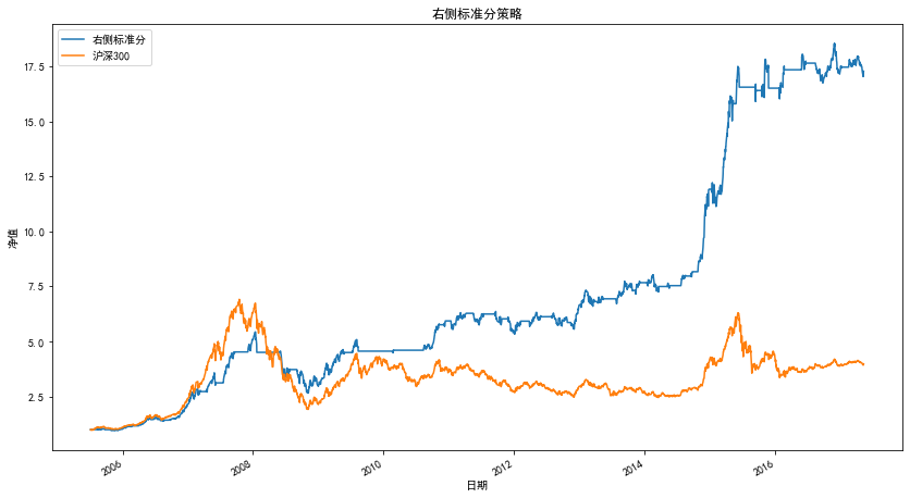
Strategic indicators
| statistic | Right standard score |
|---|---|
| net worth | 17.67 |
| Yield | 1667.22% |
| Annualized rate of return | 27.88% |
| sharpe ratio | 1.29 |
| Maximum pullback | -51.16% |
| Position days | 1638 |
| Number of transactions | 37.5 |
| Average position days | 43 |
| Profit days | 928 |
| Loss days | 710 |
| Winning rate (by day) | 56.65% |
| Average profit rate (by day) | 1.27% |
| Average loss rate (by day) | -1.22% |
| Average profit loss ratio (by day) | 1.04 |
| Profit times | 26 |
| Number of losses | 11 |
| Single maximum profit | 91% |
| Single maximum loss | -17% |
| Winning rate (by times) | 70.27% |
| Average profit rate (by time) | 15% |
| Average loss rate (by time) | -3% |
| Average profit loss ratio (by times) | 4.6 |
3.3 optimization in combination with market conditions
Based on the four indicators of the relative strength of resistance support introduced above, the trading strategies constructed by RSRS have greatly outperformed the benchmark income, but they also have a common defect: the net value has retreated sharply during the stock disaster in 2008.
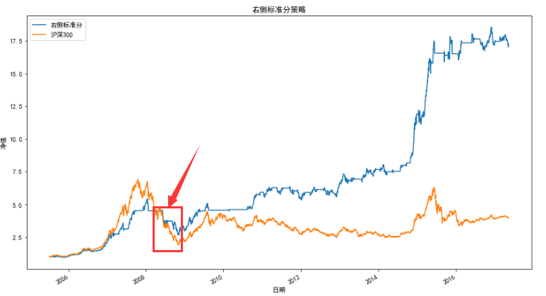
This is because according to the logic of the relative strength index of resistance support, the strategic probability is to open and close positions on the left. (the left side here refers to the falling stage when the stock price presents a "V" shape, not the left side mentioned in the right standard time sharing discussed above). However, when the market is in a bear market, if the opening forecast is wrong, it will cause serious losses.
Therefore, we expect to reduce the probability of false opening in the bear market as much as possible while ensuring the return.
The simple idea is: first judge whether the market state is in an upward or downward trend, and then build a buy and sell strategy in combination with RSRS.
3.3.1 optimization of combined moving average index
There are many indicators to help us judge the recent market status, such as MA, MACD, etc. Here, we use the relative size of the 20 day moving average of the current day and the 20 day moving average of the previous 3 days to judge the recent market state.
The optimized trading strategy is:
1. Calculate the RSRS standard sub index buying and selling signal.
- If the index sends a buy signal and the value of MA(20) of the previous day is greater than that of MA(20) of the previous three days, then buy.
- If the indicator sends a sell signal, sell your holdings.
Policy code
RSRS Index matching price data optimization strategy
def cal_ma_beta(df,n):
    df1 = cal_stdbeta(df,n)
    df1['position'] = 0
    df1['flag'] = 0
    df1['net_asset_value'] = 0
    position = 0

#beta means no data in the first 17 days (n=18) and ma20 means no data in the first 20 days
    for i in range(5,len(df1.index)-1):
        if df1['stdbeta'].iloc[i] > 0.7 and df1['ma20'].iloc[i-1]>df1['ma20'].iloc[i-3] and position == 0:
            df1['flag'].iloc[i] = 1
            df1['position'].iloc[i+1] = 1
            position = 1
        elif df1['stdbeta'].iloc[i] < -0.7 and df1['ma20'].iloc[i-1]<df1['ma20'].iloc[i-3] and position == 1:
            df1['flag'].iloc[i] = -1
            df1['position'].iloc[i+1] = 0
            position = 0
        else:
            df1['position'].iloc[i+1] = df1['position'].iloc[i]
    df1['net_asset_value'] = (1+df1.close.pct_change(1).fillna(0)*df1.position).cumprod()
    return df1
Net worth curve
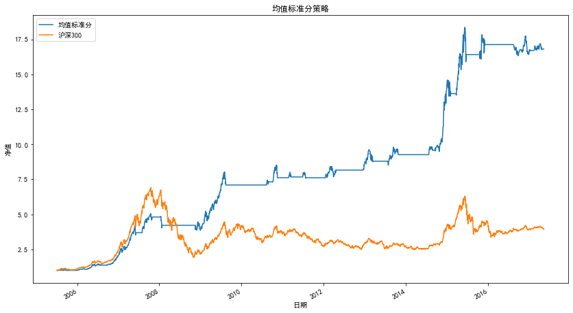
Strategic indicators
| statistic | Mean optimization standard score strategy |
|---|---|
| net worth | 16.91 |
| Yield | 1591.22% |
| Annualized rate of return | 27.36% |
| sharpe ratio | 1.48 |
| Maximum pullback | -23.61% |
| Position days | 1638 |
| Number of transactions | 37.5 |
| Average position days | 43 |
| Profit days | 714 |
| Loss days | 470 |
| Winning rate (by day) | 60.30% |
| Average profit rate (by day) | 1.24% |
| Average loss rate (by day) | -1.24% |
| Average profit loss ratio (by day) | 1 |
| Profit times | 26 |
| Number of losses | 11 |
| Single maximum profit | 91% |
| Single maximum loss | -17% |
| Winning rate (by times) | 70.27% |
| Average profit rate (by time) | 15% |
| Average loss rate (by time) | -3% |
| Average profit loss ratio (by times) | 4.6 |
3.3.2 optimization combined with transaction volume correlation
In addition to confirming the current market trend directly from the recent historical price, many published studies show that there is an obvious positive correlation between the rise and fall of the market and the trading volume. Drawing on similar ideas, we try to filter misjudgment signals by using the correlation between transaction volume and corrected standard score. Only when the correlation is positive can we consider the trading signal as a reasonable signal.
The optimized strategy is
- Calculate the trading signal of RSRS standard sub index.
- If the indicator sends a buy signal and the correlation between the trading volume of the previous 10 days and the revised standard score is positive, then buy.
- If the indicator sends a sell signal, sell your holdings.
Policy code
#Optimization based on the correlation between RSRS index and transaction volume
def cal_vol_beta(df,n):
    df1 = cal_stdbeta(df,n)

    df1['position'] = 0
    df1['flag'] = 0
    df1['net_asset_value'] = 0
    position = 0

    for i in range(10,len(df1.index)-1):

        pre_volume = df1['volume'].iloc[i-10:i]
        series_beta = df1['stdbeta'].iloc[i-10:i]
        #The data required to calculate the correlation coefficient is in series format
        corr = series_beta.corr(pre_volume,method = 'pearson')
        if df1['stdbeta'].iloc[i] > 0.7 and corr > 0 and position == 0:
            df1['flag'].iloc[i] = 1
            df1['position'].iloc[i+1] = 1
            position = 1
        elif df1['stdbeta'].iloc[i] < -0.7 and position == 1:
            df1['flag'].iloc[i] = -1
            df1['position'].iloc[i+1] = 0
            position = 0
        else:
            df1['position'].iloc[i+1] = df1['position'].iloc[i]

    df1['net_asset_value'] = (1+df1.close.pct_change(1).fillna(0)*df1.position).cumprod()
    return df1
Net worth curve

Strategic indicators
| statistic | Trading volume optimization standard score strategy |
|---|---|
| net worth | 13.97 |
| Yield | 1296.64% |
| Annualized rate of return | 25.10% |
| sharpe ratio | 1.57 |
| Maximum pullback | -22.29% |
| Position days | 916 |
| Number of transactions | 40 |
| Average position days | 22 |
| Profit days | 548 |
| Loss days | 368 |
| Winning rate (by day) | 59.83% |
| Average profit rate (by day) | 1.29 |
| Average loss rate (by day) | -1.16 |
| Average profit loss ratio (by day) | 1.11 |
| Profit times | 27 |
| Number of losses | 13 |
| Single maximum profit | 79% |
| Single maximum loss | -16% |
| Winning rate (by times) | 67.50% |
| Average profit rate (by time) | 13% |
| Average loss rate (by time) | -4% |
| Average profit loss ratio (by times) | 3.71 |
3.4 summary of strategy results
Now give the net worth curve and statistics of all RSRS strategies
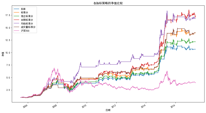
| statistic | Slope | Standard score | Revised standard score | Right standard score | Mean optimization standard score | Optimized trading volume standard |
|---|---|---|---|---|---|---|
| net worth | 10.66 | 13.93 | 12.15 | 17.67 | 16.91 | 13.97 |
| Yield | 965.73% | 1292.70% | 1115.40% | 1667.22% | 1591.22% | 1296.64% |
| Annualized rate of return | 21.92% | 25.07% | 23.47% | 27.88% | 27.36% | 25.10% |
| sharpe ratio | 1.16 | 1.28 | 1.19 | 1.29 | 1.48 | 1.57 |
| Maximum pullback | -50.26% | -50.26% | -51.28% | -51.16% | -23.61% | -22.29% |
| Position days | 1184 | 1298 | 1397 | 1638 | 1638 | 916 |
| Number of transactions | 21 | 67 | 46 | 37.5 | 37.5 | 40 |
| Average position days | 56 | 19 | 30 | 43 | 43 | 22 |
| Profit days | 747 | 741 | 790 | 928 | 714 | 548 |
| Loss days | 575 | 557 | 607 | 710 | 470 | 368 |
| Winning rate (by day) | 56.51% | 57.09% | 56.55% | 56.65% | 60.30% | 59.83% |
| Average profit rate (by day) | 1.31% | 1.32% | 1.30% | 1.27% | 1.24% | 1.29 |
| Average loss rate (by day) | -1.25% | -1.25% | -1.25% | -1.22% | -1.24% | -1.16 |
| Average profit loss ratio (by day) | 1.05 | 1.06 | 1.05 | 1.04 | 1 | 1.11 |
| Profit times | 16 | 40 | 32 | 26 | 26 | 27 |
| Number of losses | 5 | 26 | 14 | 11 | 11 | 13 |
| Single maximum profit | 170% | 91% | 76% | 91% | 91% | 79% |
| Single maximum loss | -12% | -41% | -18% | -17% | -17% | -16% |
| Winning rate (by times) | 76.19% | 60.61% | 69.57% | 70.27% | 70.27% | 67.50% |
| Average profit rate (by time) | 25% | 18% | 11% | 15% | 15% | 13% |
| Average loss rate (by time) | -3% | -9% | -3% | -3% | -3% | -4% |
| Average profit loss ratio (by times) | 7.86 | 2.05 | 3.3 | 4.6 | 4.6 | 3.71 |
4. Summary
This paper basically reproduces the research content of Everbright Securities - market timing based on the relative strength of resistance support (RSRS), and obtains the results similar to the original research report.
Shortcomings of this paper:
1. Transaction costs are not considered. The original research report also gave the results of various strategies under different transaction costs, and the net value decreased slightly.
2. The performance of strategies when selecting different N and M is not given.
5. Author
He Baisheng, School of economics and management, Weihai campus, Harbin Institute of Technology
Cai Jinhang, School of computer science and technology, Weihai campus, Harbin Institute of Technology
Write at the end
We are students of domestic colleges and universities and beginners of quantitative investment. Our school is not reopened in northern Qing Dynasty, nor does it have a financial engineering laboratory. At the same time, it is located in a third tier town. Therefore, it is difficult for us to obtain quantitative internship opportunities during our school period, but we look forward to communicating and communicating with the industry.
Cai Jinhang is one of us. When looking for the quantitative internship in summer, he received the written examination invitation from several private placement and brokerage metalworking groups. The written examination content is to reproduce a metalworking Research Report within a given time. Inspired, Cai found that reproducing the metalworking research report is not only a good way for us to learn quantitative strategies, exercise program design ability, but also a good way to communicate with the industry.
At the suggestion of CAI, we started the creation of the reproduction series of the research report, recorded our learning process, shared our creative content, and communicated, studied and made progress with readers.
Our level is limited, and the content of our creation will inevitably have errors or imprecise content. We welcome readers' criticism and correction.
If you are interested in our content, please contact us: cai_jinhang@foxmail.com