When I see the logistic regression classifier, my first reaction is that it's not a statistical logistic regression. In fact, it's the same. I've written about the practice of logistic regression before. I'll write it again under the framework of machine learning today.
logistic regression is a supervised learning method that predicts class membership
What is logistic regression?
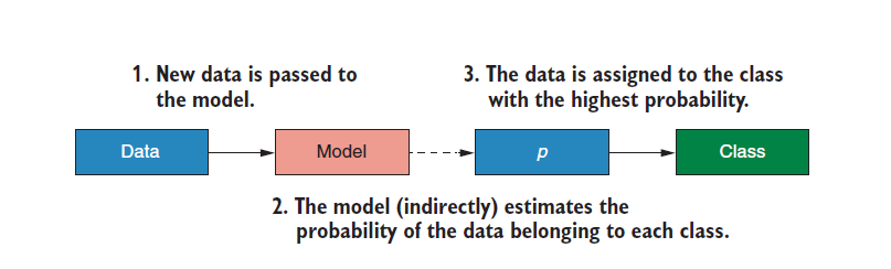
Logistic classifier is classified by probability. The algorithm will predict the probability of an individual belonging to a certain class according to the predictive variables, and then divide the individual into the class with the highest probability. When our response variable is binary logistic expression, we call it binomial logistic expression, and when we are multi classified, we call it multinomial logistic expression.
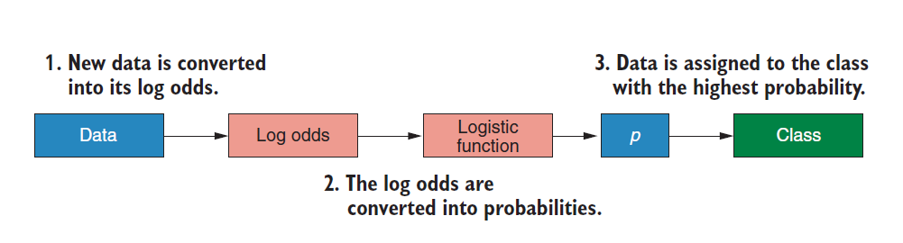
The classification process of logistic classifier is as follows:
How is the above probability calculated? Let's follow me and disassemble it with a practical example:
If you are an expert in cultural relics identification, there are a number of cultural relics that need you to identify their authenticity. We only know the copper content of cultural relics. Previous experience tells us that cultural relics in places with copper content are more likely to be fake. Now you want to train a model to predict the authenticity of cultural relics according to the copper content (second classification problem).
We can draw the relationship between the authenticity of cultural relics and copper content according to the previous data:
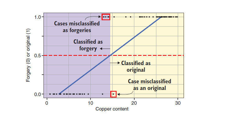
Let's take a closer look at the above figure. We have a blue line, which is the fitting line of general linear regression. If I take the copper content that makes the ordinate of the blue line take 0.5 as the limit, and think that those below 0.5 are fake cultural relics and those above 0.5 are real cultural relics, then I must be unqualified as an expert (the above three cultural relics have been wrongly classified), I need to train a better model.
For example, the fitting of logistic regression classifier to the same data is shown in the figure below:
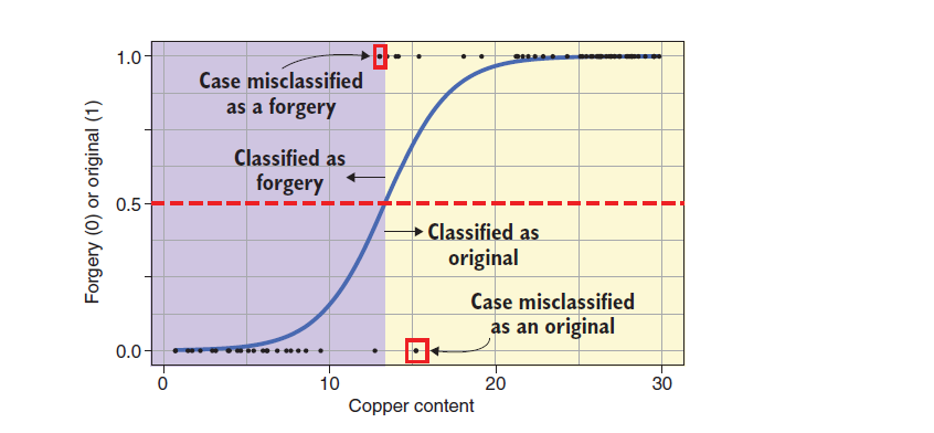
Let's look at the fitting of logistic regression classifier. At this time, if I take the copper content that makes the vertical coordinate of the blue line take 0.5 as the limit and think that those below 0.5 are fake cultural relics and those above 0.5 are real cultural relics, then my expert is much better than the expert just now (there are only two wrong points in total), Moreover, the logistic regression classifier maps all the values of y corresponding to x to the range of 0 to 1, which is very practical. Just that linear classification, too large or too small copper content will make the value of y exceed the range of practical significance.
Although the S-shaped curve of this logistic regression classifier performs well in the task of identifying the authenticity of cultural relics, what is the practical significance of this line?
This S-shaped curve is the value of log odd. It is estimated that someone is confused. Keep looking down.
Then I will introduce the concept of log odd
But before that, you have to write odds to take care of the students with weak foundation
Look at the following formula:

Remember that the probability of odds is the ratio of true to false

This is often seen in epidemiology. Odds is a very important indicator representing the occurrence of an event:
They tell us how much more likely an event is to occur, rather than how likely it is not to occur.
Basically, every Xiaobai understands the meaning of probability p, but the value of probability p can only be 0 to 1, but the value of odds extends to the whole set of positive numbers.
Returning to the example of identifying the authenticity, we try to visualize the odds and copper content of cultural relics, as shown in the following figure:
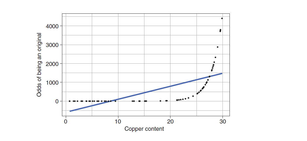
You can see that our odds is indeed from 0 to positive infinity, but the relationship between copper content and odds with real cultural relics is a curve, which is not easy to fit, so we naturally think of variable conversion.
Tell me, what is the most common variable conversion method?
log conversion
It's too smart. It has been converted into log odd
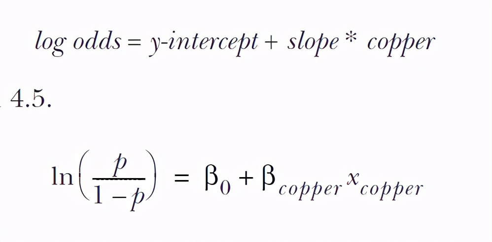
So we have this converted formula (this is called logit function, which is the connection function of logistics regression):

OK, now let's work out the relationship between odds and copper content after log conversion:
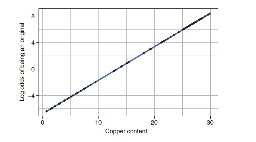
The miracle of perfect fitting appears. Through the whole process above, we really turn the classification problem into a general linear regression problem. The core is the logit function. Let's have a good experience.
One of the advantages of converting to linear relationship is that it is intuitive and simple. More importantly, we can include many other predictive variables by converting to linear relationship
Additionally, having a linear relationship means that when we have multiple predictor variables, we can add their contributions to the log odds together to get the overall log odds of a painting being an original, based on the information from all of its predictors.
Finally, to sum up, in the logistic regression classifier, our idea is to start from the probability p, but p can only be taken in the range of 0 to 1. Therefore, we introduce the concept of odds from P, successfully expand the value of response variables to the positive real number set, and then make the linear relationship between prediction variables and response variables through the log conversion of multiple odds. The logic classifier algorithm is probably such a process. Therefore, you should understand that the fitting result of our prediction variables is actually logods, and the algorithm will convert logods back to probability p against the above process to realize the prediction.
The whole process is as follows:
There are also several formulas to stick to you again:
logistics classifier practice
Just mastering the theory is not enough. Continue our example practice. Now you have the passenger information of Titanic cruise ship in your hand. What you need to do now is to train a logistics classifier to predict the life and death of passengers according to the characteristics of passengers.
Our data set is about this long:
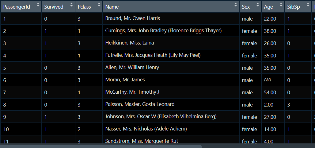
This data set has a total of 12 variables and needs a series of preprocessing, including Feature extraction, Feature creation and feature selection. Because data preprocessing is not the focus of this paper, it will not be expanded here. After processing, we get the data set as follows:
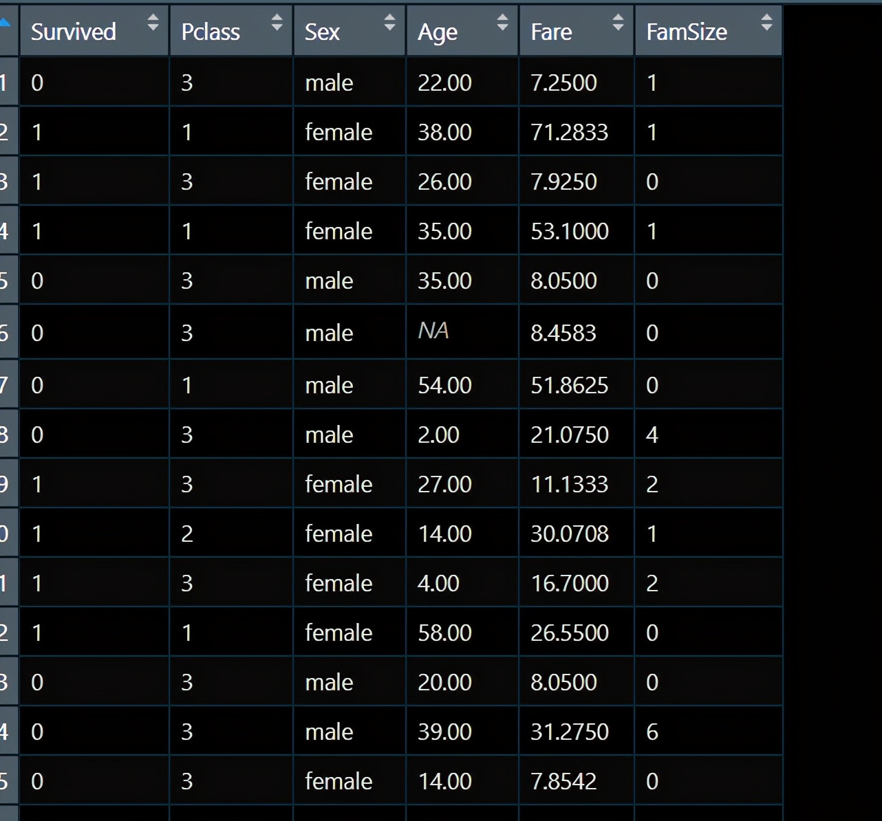
Survived is the survival of passengers, which is our response variable, and the rest are our predictive variables.
After data processing, the first step is usually visualization
<span style="color:#222222"><code>titanicUntidy <- gather(titanicClean, key = <span style="color:#00753b">"Variable"</span>, value = <span style="color:#00753b">"Value"</span>,
                        -<span style="color:#a82e2e">Survived</span>)
titanicUntidy %>%
<span style="color:#114ba6">filter</span>(<span style="color:#a82e2e">Variable</span> != <span style="color:#00753b">"Pclass"</span> & <span style="color:#a82e2e">Variable</span> != <span style="color:#00753b">"Sex"</span>) %>%
ggplot(aes(<span style="color:#a82e2e">Survived</span>, <span style="color:#114ba6">as</span>.numeric(<span style="color:#a82e2e">Value</span>))) +
facet_wrap(~ <span style="color:#a82e2e">Variable</span>, scales = <span style="color:#00753b">"free_y"</span>) +
geom_violin(draw_quantiles = <span style="color:#114ba6">c</span>(<span style="color:#a82e2e">0.25</span>, <span style="color:#a82e2e">0.5</span>, <span style="color:#a82e2e">0.75</span>)) +
theme_bw()

titanicUntidy %>%
<span style="color:#114ba6">filter</span>(<span style="color:#a82e2e">Variable</span> == <span style="color:#00753b">"Pclass"</span> | <span style="color:#a82e2e">Variable</span> == <span style="color:#00753b">"Sex"</span>) %>%
ggplot(aes(<span style="color:#a82e2e">Value</span>, fill = <span style="color:#a82e2e">Survived</span>)) +
facet_wrap(~ <span style="color:#a82e2e">Variable</span>, scales = <span style="color:#00753b">"free_x"</span>) +
geom_bar(position = <span style="color:#00753b">"fill"</span>) +
theme_bw()</code></span>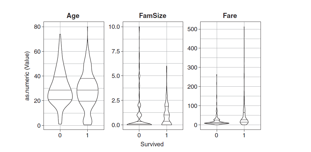
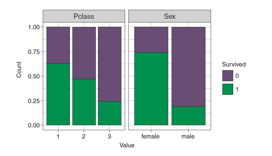
Through the single factor visualization above, you can see the relationship between the survival of passengers and various predictive variables. The figure is very simple. I won't explain it to you. Let's go directly to the model training section.
model training
The model training is still divided into three steps, the first is to set the task, the second is to set the learner, and the third is to train:
<span style="color:#222222"><code><span style="color:#114ba6">titanicTask</span> <- makeClassifTask(data = imp<span style="color:#d96322">$data</span>, target = <span style="color:#00753b">"Survived"</span>)<span style="color:#999999">#First step</span>
logReg <- makeLearner(<span style="color:#00753b">"classif.logreg"</span>, predict.type = <span style="color:#00753b">"prob"</span>)<span style="color:#999999">#Step two</span>
logRegModel <- train(logReg, titanicTask)<span style="color:#999999">#Step 3 < / span > < / code ></span>
Run the above code to train our logistics classification model logRegModel.
Then we need to do cross validation.
Cross validation
What is cross validation? If you still ask this question, please go to the previous article to review. For this example, we have a data interpolation process, so in order to stabilize the divided data set, I will carry out the same missing value interpolation process for each sampling
<span style="color:#222222"><code>logRegWrapper <span style="color:#00753b"><- makeImputeWrapper("classif.logreg",</span>
                                   cols = <span style="color:#00753b">list(Age = imputeMean()))</span>

kFold <span style="color:#00753b"><- makeResampleDesc(method = "RepCV", folds = 10, reps = 50,</span>
                          stratify = <span style="color:#00753b">TRUE)</span>
logRegwithImpute <span style="color:#00753b"><- resample(logRegWrapper, titanicTask,</span>
                             resampling = <span style="color:#00753b">kFold,</span>
                             measures = <span style="color:#00753b">list(acc, fpr, fnr))</span></code></span>
Run the above code to verify the 10% discount. The results are as follows:
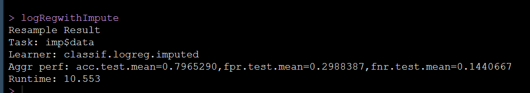
We can see the accuracy of our logistic regression classifier acc.test Mean = 0.7965290, false positive fpr test. Mean = 0.2988387, the false negative rate was FNR test. mean=0.1440667.
Interpretation of the model
Run the following code to get the coefficients of the model, and then write the explanation of the model coefficients:
<span style="color:#222222"><code><span style="color:#114ba6">logRegModelData</span> <- getLearnerModel(logRegModel)
coef(logRegModelData)</code></span>
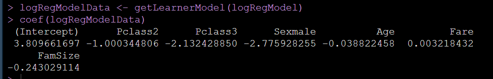
We first have an outcome item intercept, which indicates how many log odds our passengers survive when all predictive variables are 0. Of course, we are more related to the coefficients of each predictive variable β, These are two coefficients β It means that when other predictive variables remain unchanged, a predictive variable increases by one unit, and the log odd of passenger survival increases β Units.
But log odds is hard to explain, so a more friendly way is to convert log odds into odds ratio (that is, the ratio of two risks, called odds ratio), so we can convert the coefficient β These coefficients are interpreted as: β It means that when other predictive variables remain unchanged, a predictive variable increases by one unit, and the passenger survival odds increases by e relative to the reference level β Power times.
For example, if the odds of surviving the Titanic if you're female are about 7 to 10, and the odds of surviving if you're male are 2 to 10, then the odds ratio for surviving if you're female is 3.5. In other words, if you were female, you would have been 3.5 times more likely to survive than if you were male. Odds ratios are a very popular way of interpreting the impact of predictors on an outcome, because they are easily understood.
Therefore, of course, we hope that our model can also output odd ratio. The code is as follows:
<span style="color:#222222"><code><span style="color:#114ba6">exp</span>(cbind(Odds_Ratio = coef(logRegModelData), confint(logRegModelData)))</code></span>
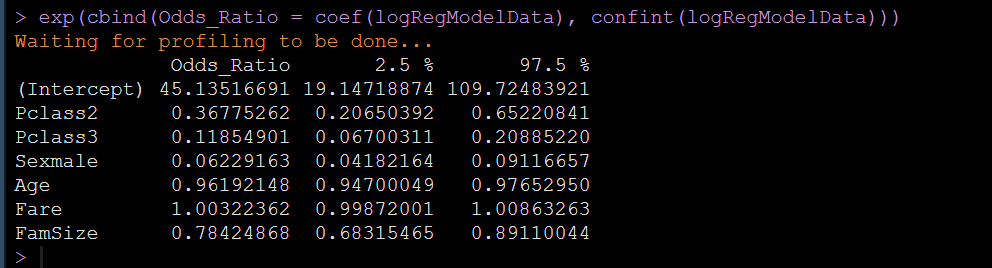
It can be seen that many odds ratios are less than 1, which indicates that the risk is reduced. For example, looking at the output of the figure, we can see that the odds ratio of male is 0.6. If we divide 1 by 0.6 = 16.7, we can explain that under the control of other predictive variables, the survival risk of male passengers is 16.7 times less than that of women.
Please understand the above text well. It is suggested to read it three times and think for three minutes.
What I just wrote is the explanation of 0 and 1 predictive variables. For the continuous predictive variables, the odds ratio can be explained as: when the other predictive variables remain unchanged, the survival risk increases by e for each unit of the variable relative to the survival risk at the reference level of the continuous variable β Power times. For example, in our example, the odds ratio of famsize is 0.78, 1 / 0.78 = 1.28. We can explain that for each additional passenger family member, the survival risk decreases by 1.28 times, or increases by 0.78 times, which is the same.
Please understand the above text well. It is suggested to read it three times and think for three minutes.
For multi category factor prediction variables, the explanations are classified as 0 and 1, so we won't write them in detail here.
Using models to make predictions
Let's not forget our original intention. We train the model to make predictions for us, so let's see how to use the newly trained logistics classifier to predict new data.
The new data is still in the titanic package. The prediction code is as follows:
<span style="color:#222222"><code>data(titanic_test, <span style="color:#114ba6">package</span> = <span style="color:#00753b">"titanic"</span>)
titanicNew <- as_tibble(titanic_test)
titanicNewClean <- titanicNew %>%
  mutate_at(.vars = c(<span style="color:#00753b">"Sex"</span>, <span style="color:#00753b">"Pclass"</span>), .funs = factor) %>%
  mutate(FamSize = SibSp + Parch) %>%
  <span style="color:#114ba6">select</span>(Pclass, Sex, Age, Fare, FamSize)

predict(logRegModel, newdata = titanicNewClean)</code></span>
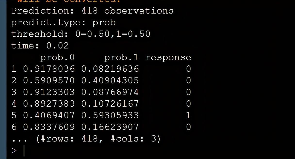
Looking at the output in the figure, we use our trained model to output the probability of survival or death of each new data and the survival outcome predicted by the model, which is perfect.
That's all for today's disassembly of the logic classifier. I'll see you later.
Summary
Today, I wrote the regression of logistics again under the framework of machine learning. I hope you can understand new things. Thank you for your patience. Your articles are written in detail and the codes are in the original text. I hope you can do it yourself. Please pay attention to the private letter and reply to the "data link" to obtain all the data and the learning materials I collected. If it's useful to you, please collect it first, then like it and forward it.
Also welcome your comments and suggestions. If you want to know what statistical methods you can leave a message under the article. Maybe I'll write a tutorial for you when I see it.