Anomaly detection

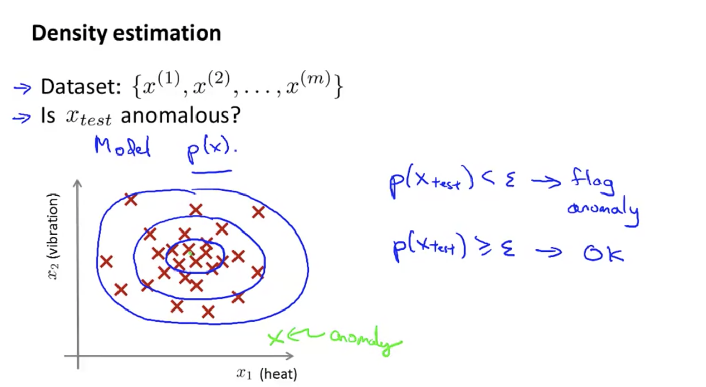
Establish a model p, which is similar to the probability of normal situation. If it is less than a certain value, it is considered to be abnormal.

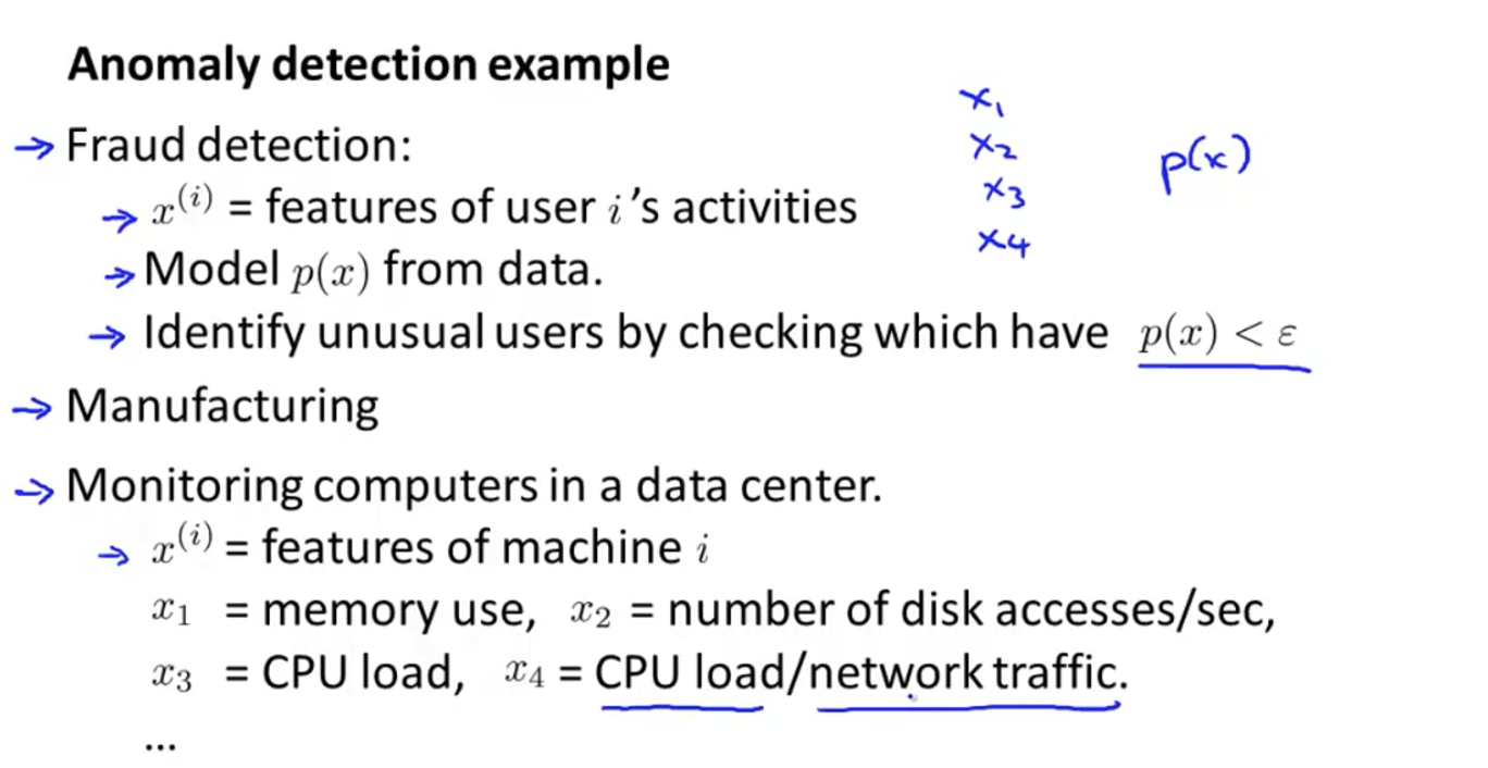
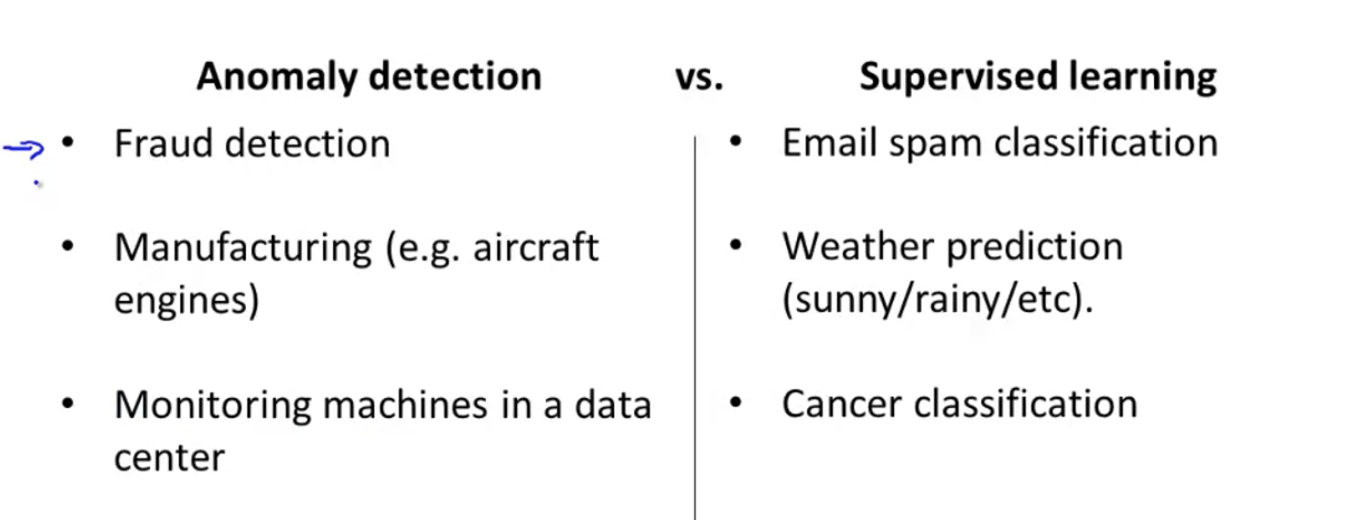
Application scenario

• Fraud detection
• Abnormal parts detection
• Data center computer working condition monitoring
  

Gaussian distribution

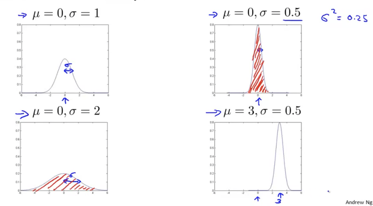
parameter estimation

Let's give you a set of x's, and let's assume that they obey a Gaussian distribution, and we calculate μ and σ Value of.

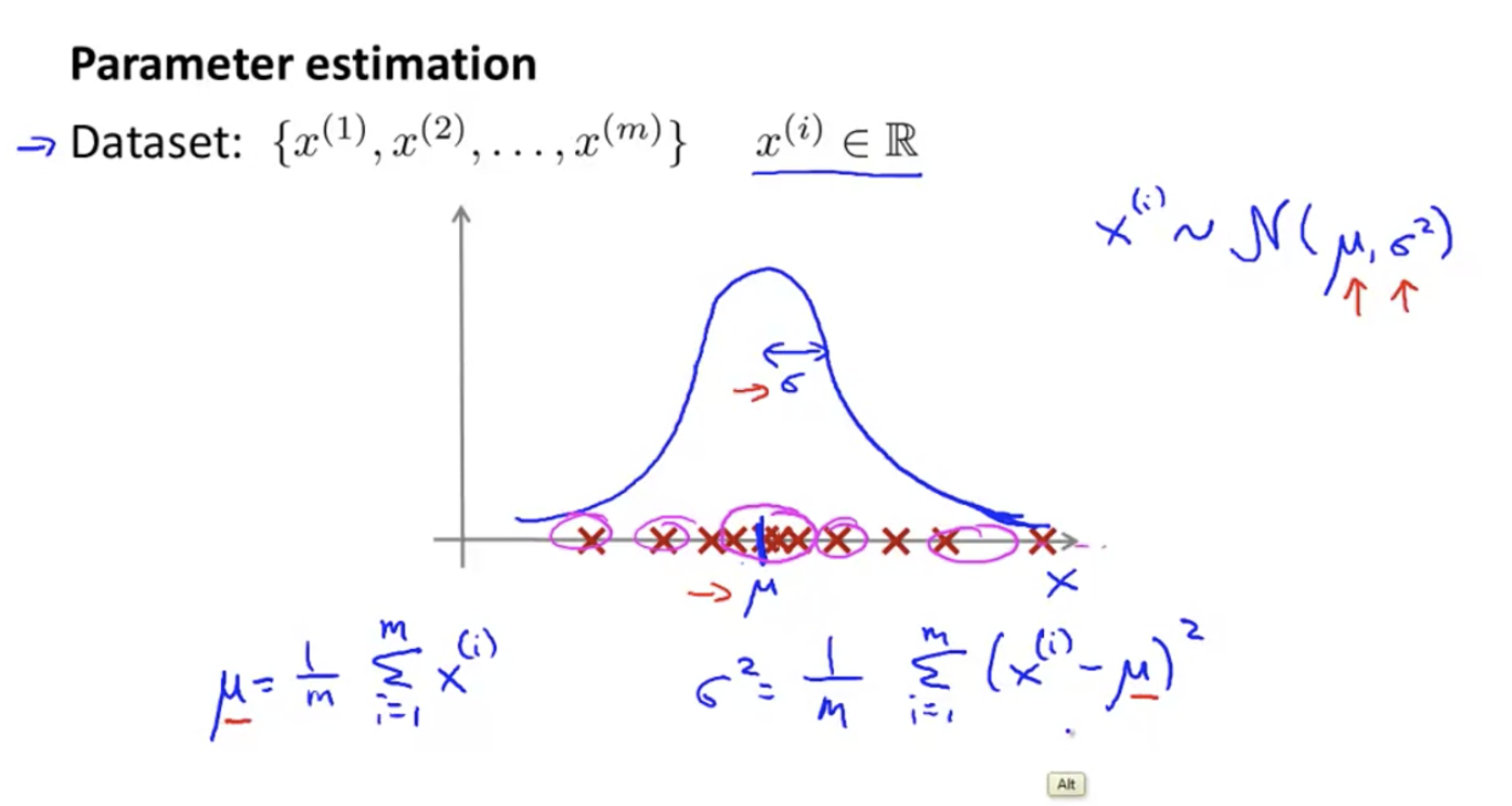
In this way, the probability of new members can be calculated.

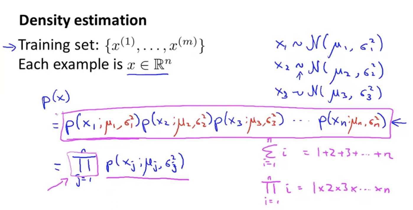
density estimation

Assuming that each characteristic of X is independent, p(x) can be calculated by the following formula.
The process of calculating p(x) is also called density estimation.

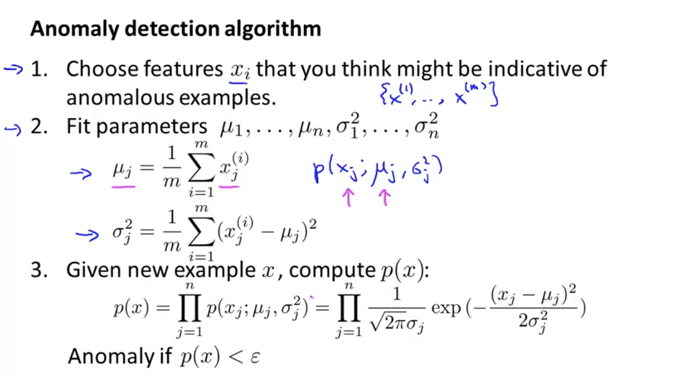
Anomaly detection algorithm

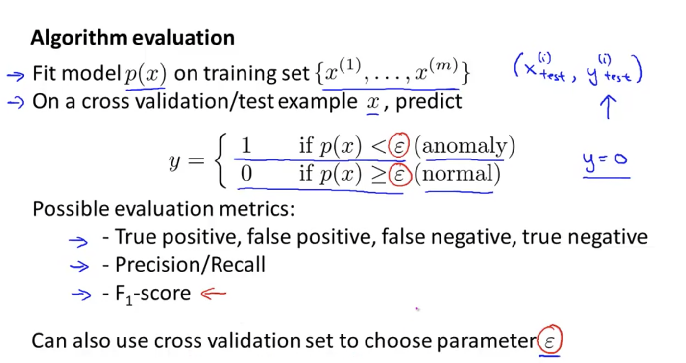
Using the density estimation of x, calculate its probability to see if it is less than a certain value.

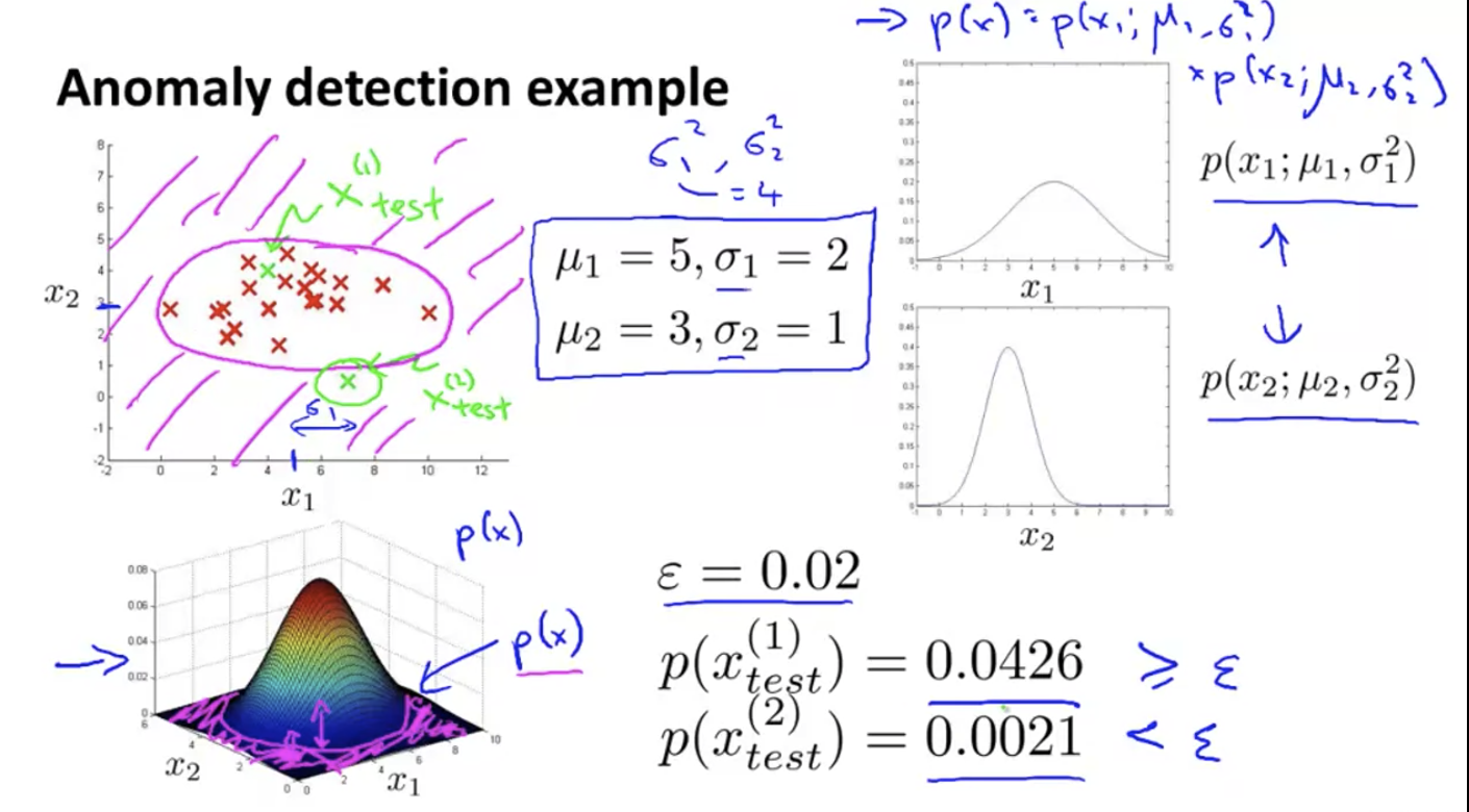
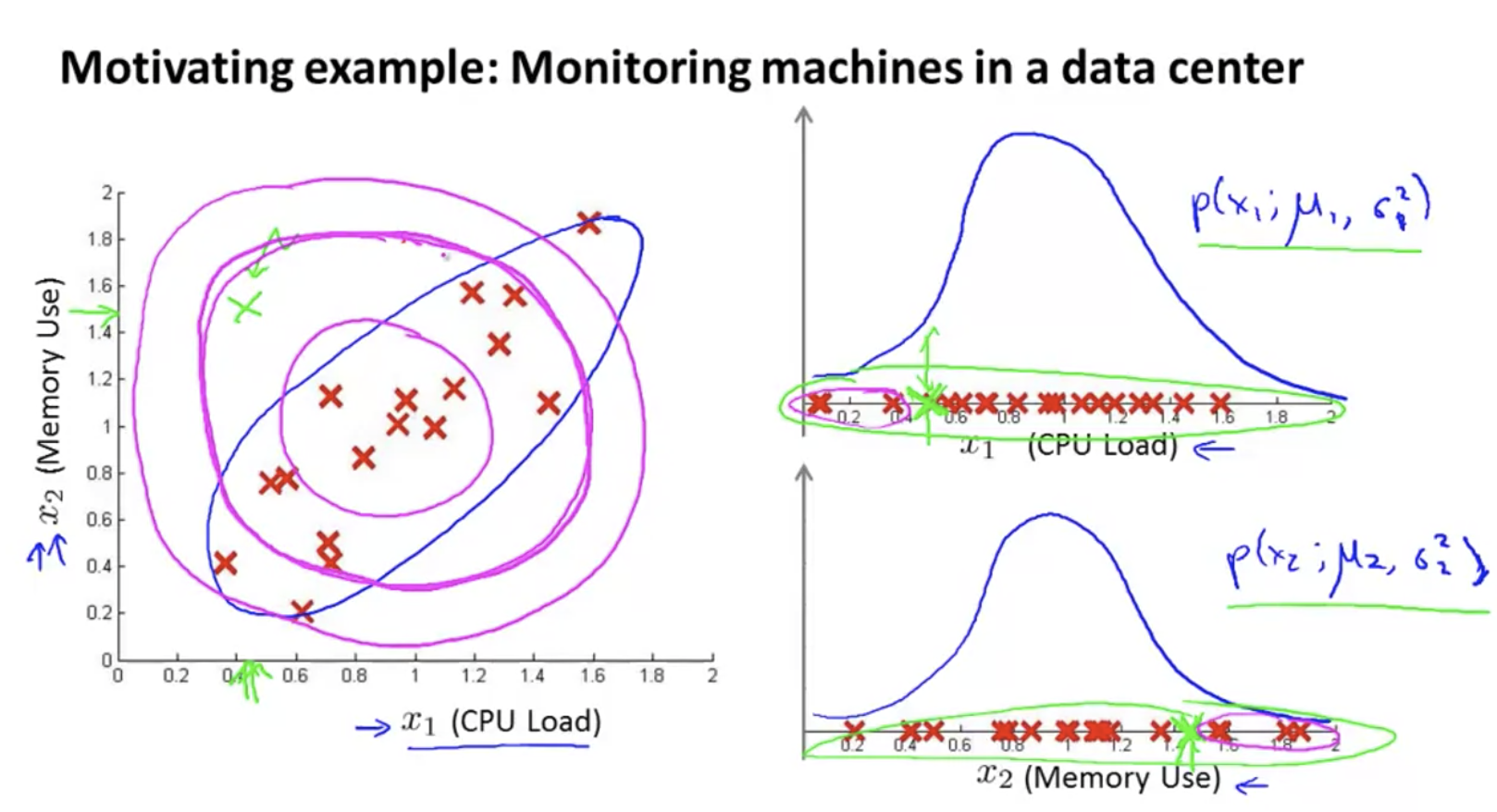
Specific examples. The Gaussian distributions of x1 and x2 are used to synthesize the three-dimensional image in the lower left corner, and the height represents the probability. The (pink) at the foot of the mountain are all low probability points, corresponding to the pink area in the upper left figure. All points falling in the pink area can be regarded as abnormal points.

How to evaluate anomaly detection algorithm

For example, how to decide which features to use?

Assuming that we have a small amount of marked data, we can allocate training set, verification set and test set as follows:
60%: 20%: 20% of normal samples
0%: 50%: 50% abnormal samples

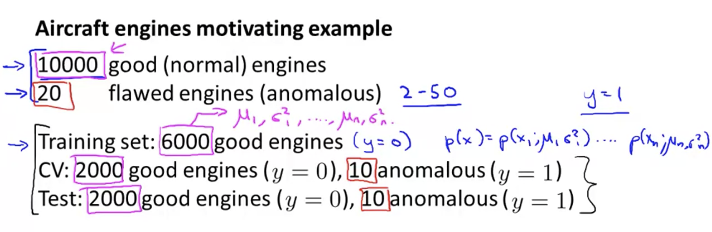
With marked data, it is similar to supervised learning.

Review the evaluation indicators for reference https://cloud.tencent.com/developer/article/1486764:

1. Confusion matrix
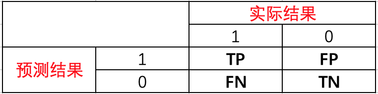
Before introducing each indicator, let's take a look at the confusion matrix. If there is a dichotomous problem now, there will be the following four situations when the predicted results are combined with the actual results.

TP, FP, FN and TN can be understood as

TP: the predicted value is 1, the actual value is 1, and the prediction is correct.
FP: predicted as 1, actual as 0, prediction error.
FN: predicted as 0, actual as 1, prediction error.
TN: the predicted value is 0, the actual value is 0, and the prediction is correct.

2. Accuracy
Firstly, the definition of accuracy is given, that is, the percentage of correct prediction results in the total samples. The expression is

Although the accuracy rate can judge the overall accuracy rate, it can not be used as a good indicator to measure the results in the case of unbalanced samples. For example, in the sample set, there are 90 positive samples and 10 negative samples. The samples are seriously unbalanced. In this case, we only need to predict all samples as positive samples, and we can get 90% accuracy, but it is completely meaningless.

3. Accuracy
Precision refers to the prediction result, which means the probability of actually being a positive sample among all the predicted positive samples. The expression is

Accuracy and accuracy look similar, but they are two completely different concepts. The accuracy rate represents the prediction accuracy in the positive sample results, and the accuracy rate represents the overall prediction accuracy, including positive samples and negative samples.

4. Recall rate
Recall refers to the original sample, which means the probability of being predicted as a positive sample in the actual positive sample. The expression is

Let's take a simple example to see the accuracy rate and recall rate. Suppose there are 10 articles in total, of which 4 are what you are looking for. According to your algorithm model, you found 5 articles, but in fact, of these 5 articles, only 3 are what you really want to find.

Then the accuracy rate of the algorithm is 3 / 5 = 60%, that is, three of the five articles you are looking for are really right. The recall rate of the algorithm is 3 / 4 = 75%, that is, you find three of the four articles you need to find. Whether to take the accuracy rate or the recall rate as the evaluation index needs to be determined according to the specific problems.

5.F1 score
Precision and recall are also called precision and recall, which can be represented by P-R diagram

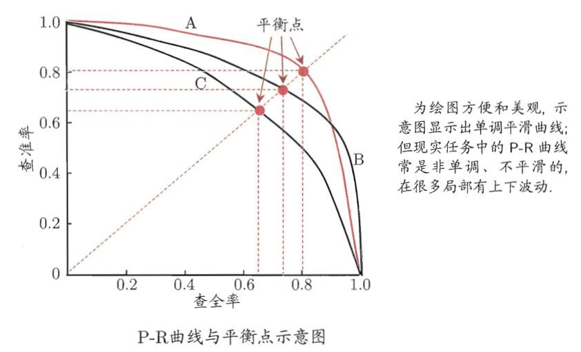
We hope that the accuracy rate and recall rate are high, but the reality needs to be weighed.
The F1 score considers both accuracy and recall to achieve the highest balance at the same time. F1 fraction expression is

In the P-R curve above, the equilibrium point is the fraction of F1 value.

In the anomaly detection algorithm, it is equivalent to having a data set with high inclination, which should be evaluated by accuracy, recall and F1 score.

Also use the validation set to select parameters ε.

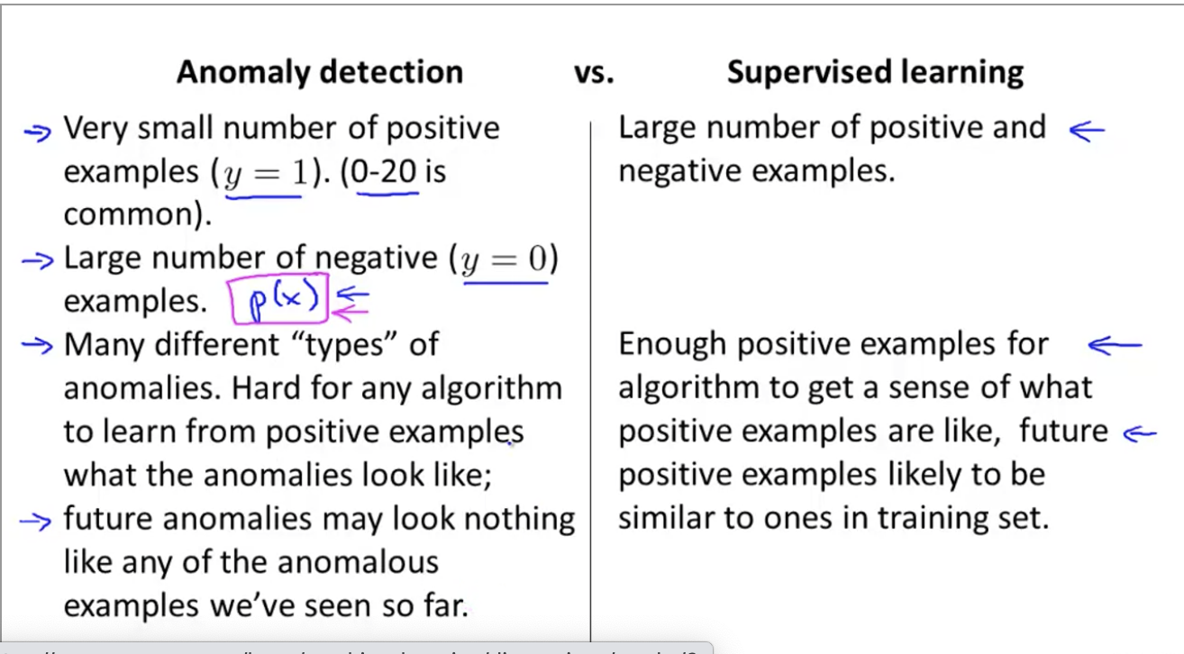
The difference between anomaly detection and supervised learning

• The number of positive samples (outliers) for anomaly detection is particularly small;
• The positive samples of anomaly detection are various and difficult to fit;
• The test set of anomaly detection may be more unreasonable and difficult to predict;

Application scenario:

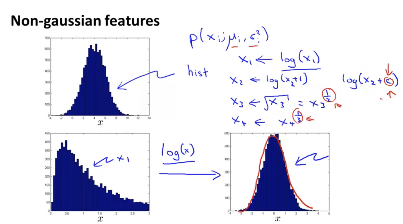
How to select features

The hist histogram can be used to see whether the data distribution roughly conforms to the normal distribution.

For the Gaussian distribution with deviation, some transformations can be made to make it more consistent with the Gaussian distribution:

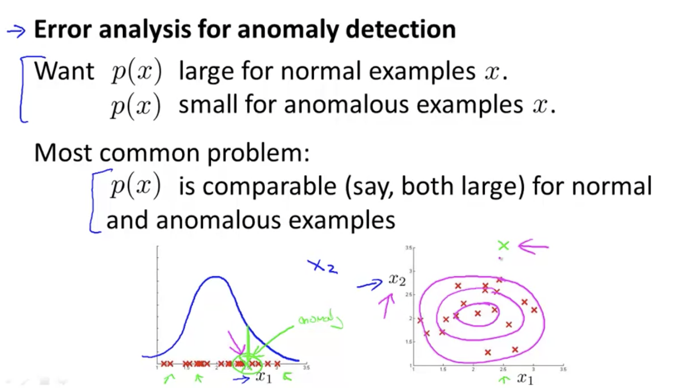
Next, how to select features? It is similar to the cross validation process of supervised learning.

After verification, if you find that the result is not good (left figure), consider how to add a feature to make the result better (right figure).

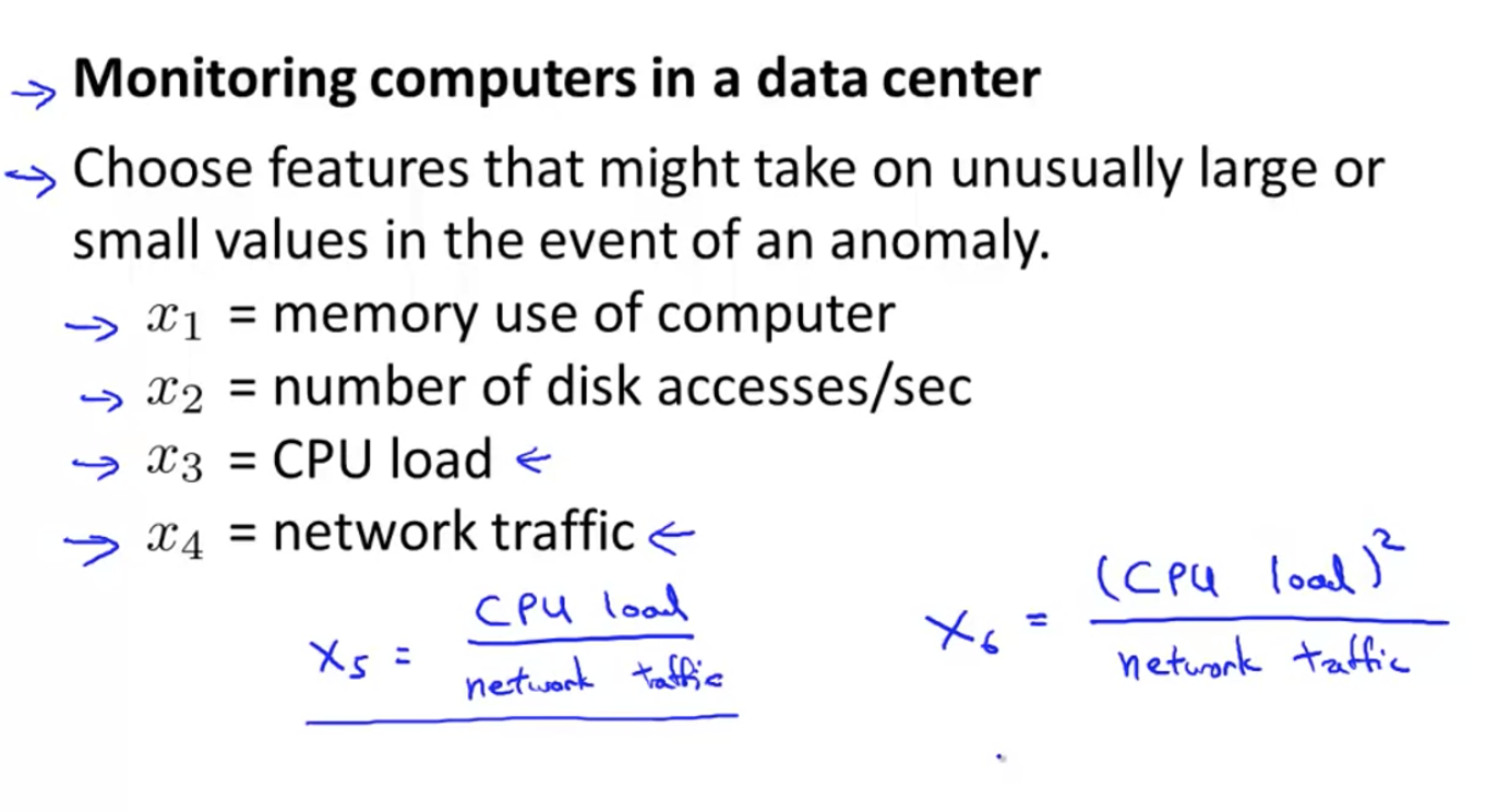
Example: Data Center host monitoring

Sometimes it may fall into a dead cycle. For example, if the CPU of a web server is too high, but the network traffic remains unchanged, a feature X5 or X6 can be added:

Multivariate anomaly detection

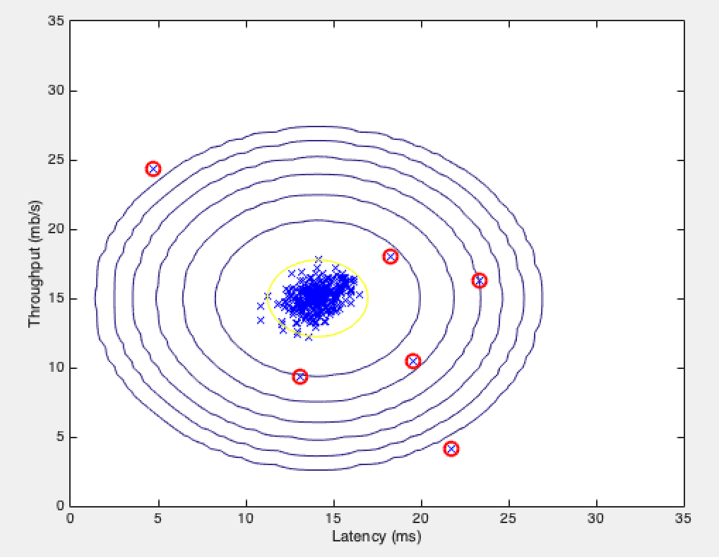
Separately, there is no problem with low CPU usage and high memory occupation; But the combination of the two is actually problematic.

But ordinary anomaly detection draws a pink concentric circle, and the green dot on the upper left cannot be detected.

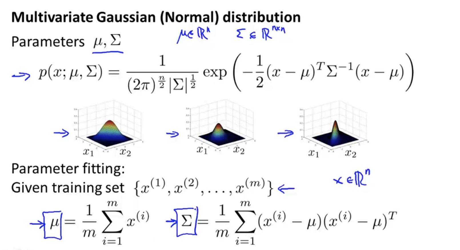
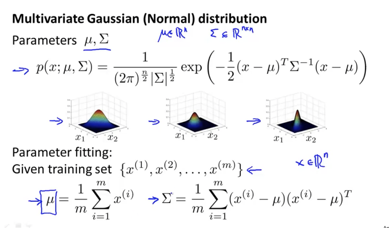
Instead of separately calculating p(x1), p(x2)... Of each feature, directly calculate p(x):

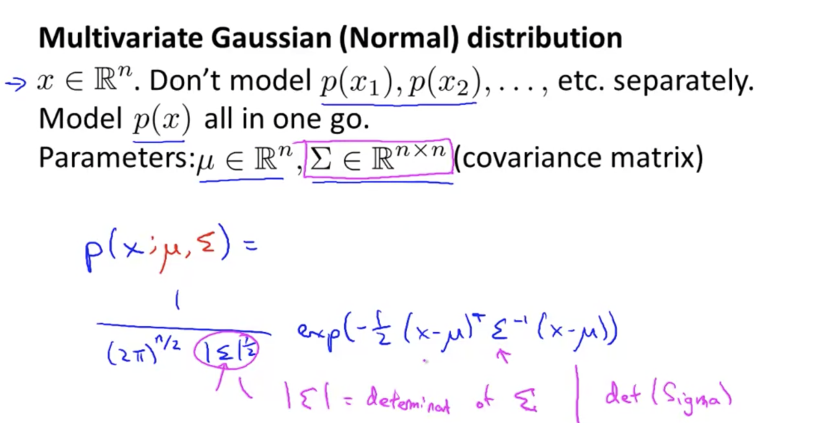
Among them| Σ| It's a determinant.

Determinant: determinant, which is a numeric value. Represents the volume of n-dimensional geometry.

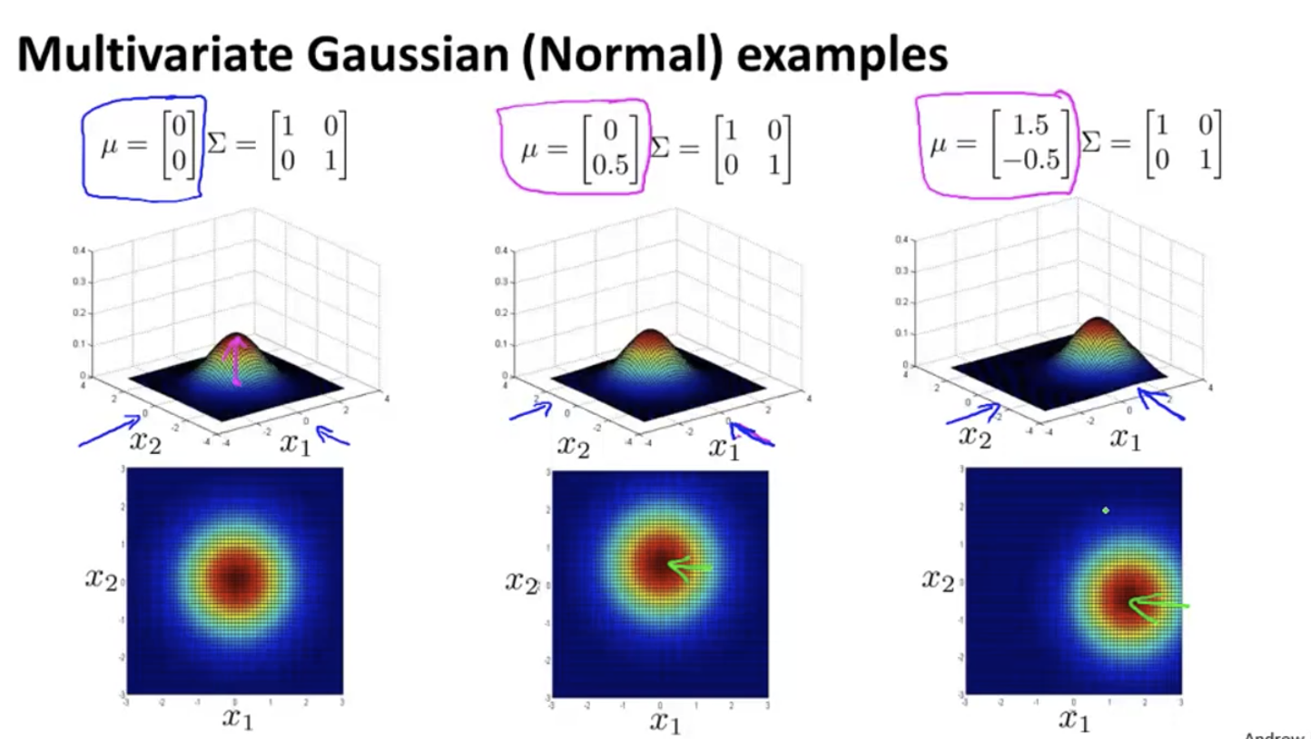
change Σ Column K of is to modify the variance of dimension k:

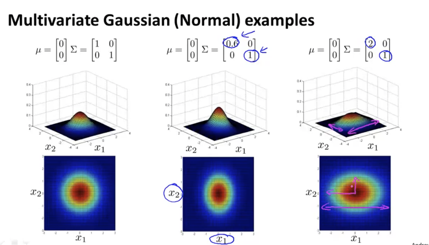
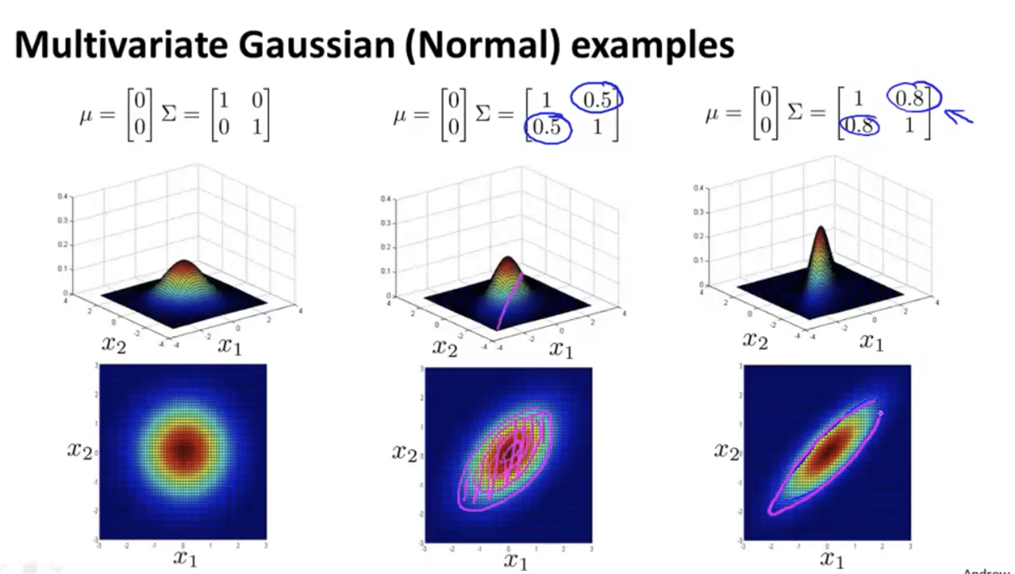
Modifying the left oblique value has the following effects: x1 and x2 are positively correlated, and the probability is large when x1 and x2 are both large:

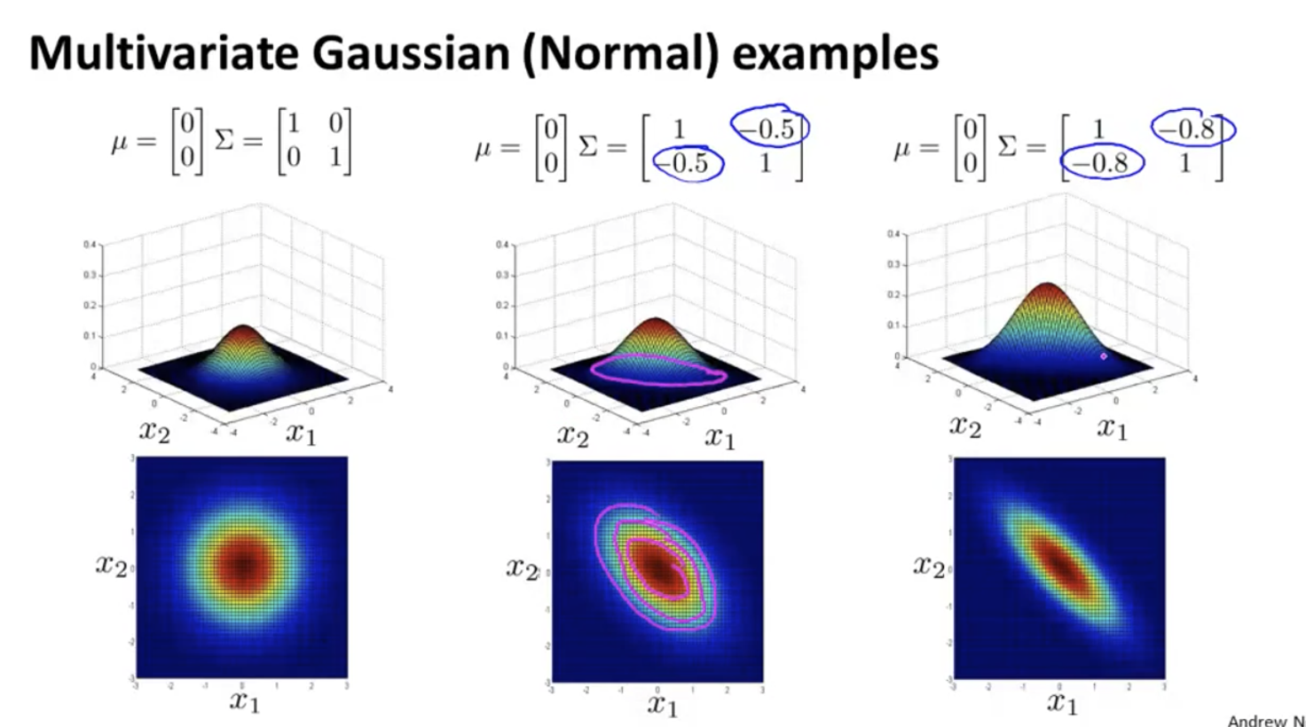
When the value of left oblique is negative, x1 and x2 are negatively correlated:


How to calculate the of multivariable Gaussian segment μ and Σ:

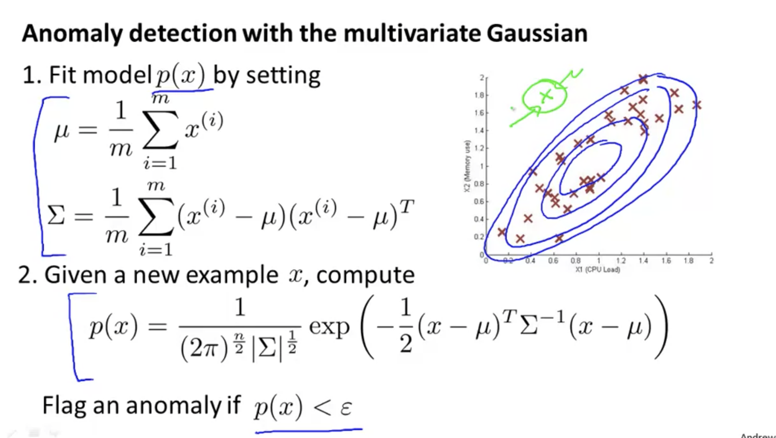
Multivariate anomaly detection uses Gaussian distribution

Multivariable anomaly detection algorithm, calculated using the following method μ and Σ:

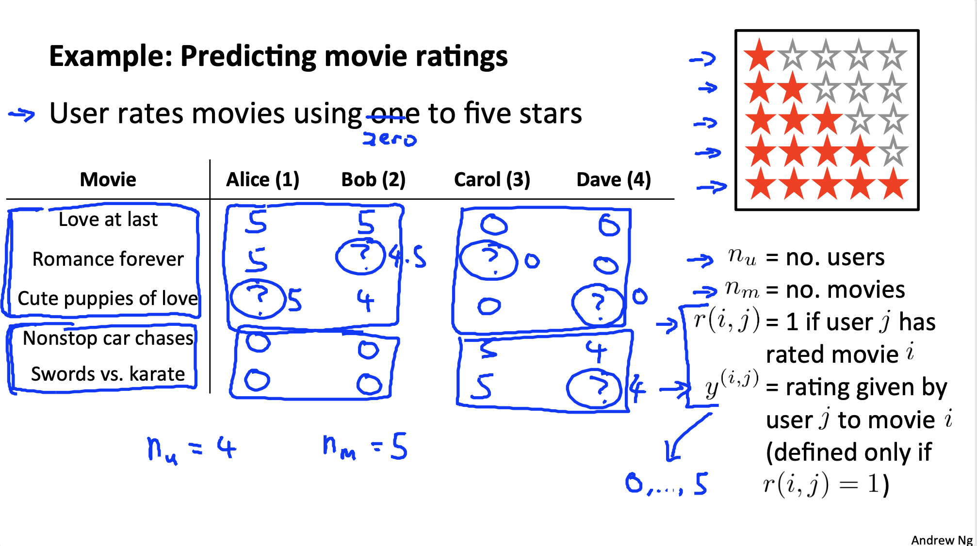
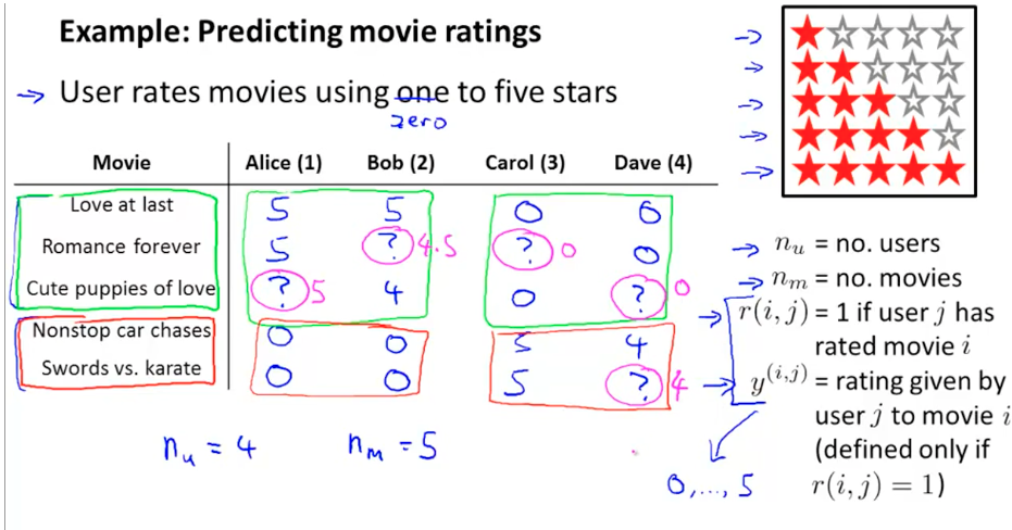
Recommendation system

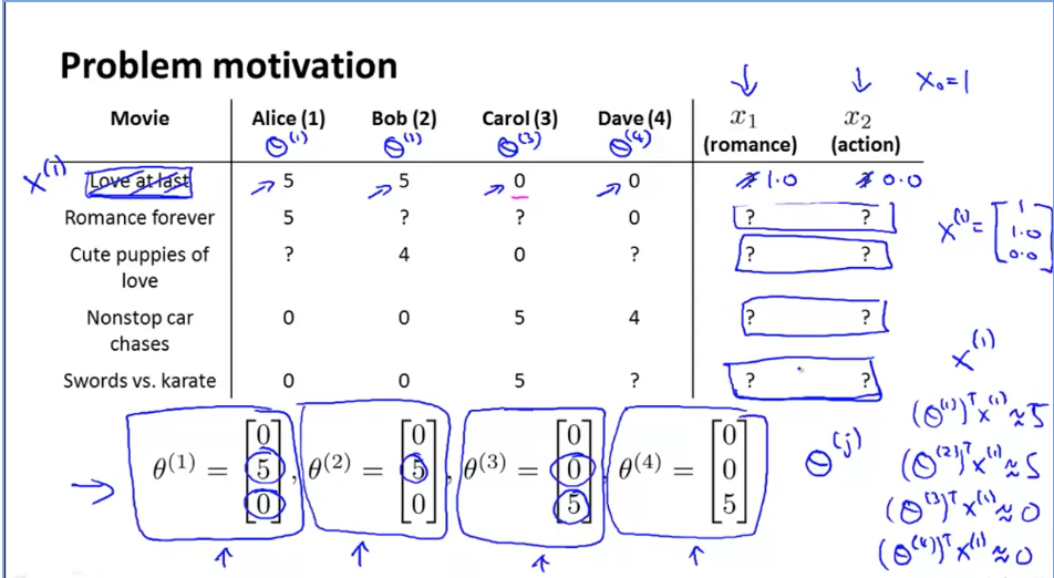
Problem definition: film review prediction

Content based recommendation

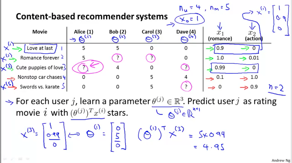
Optimization objectives, based on linear regression:

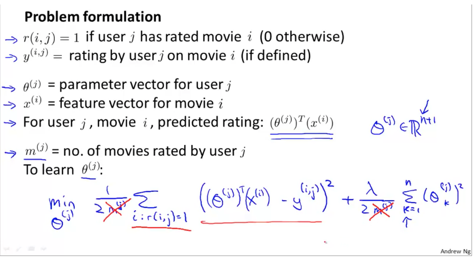
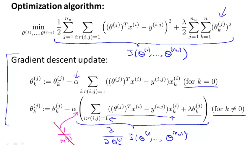
Of course, the training recommendation system needs to consider and optimize all at the same time θ， That is, consider the feelings of all users:

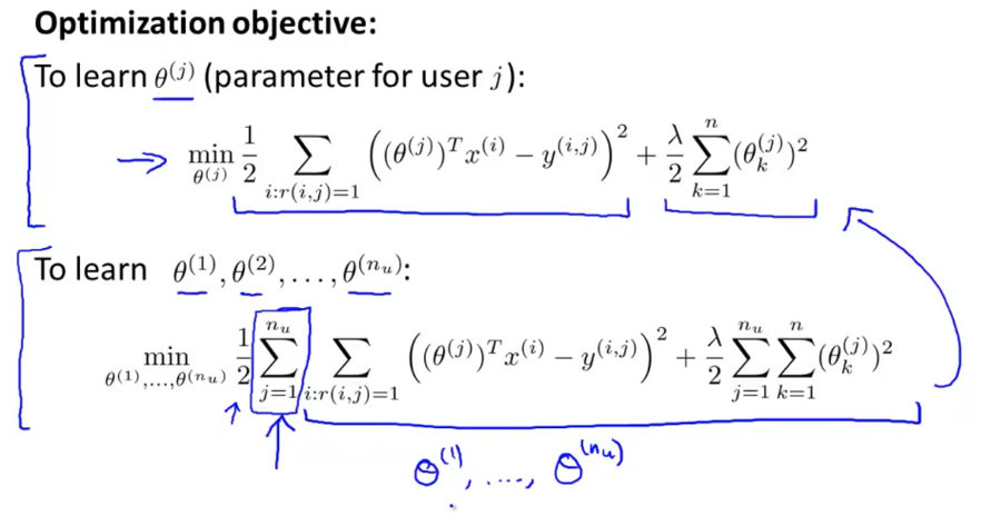
The optimization function is as follows, which is different from ordinary linear regression:

Collaborative recommendation

Sometimes know θ (user preferences for various types of movies), do not know x (type of movie).

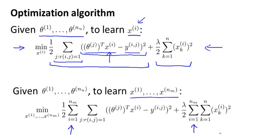
Can pass θ And y (user's rating table for the film), find x:

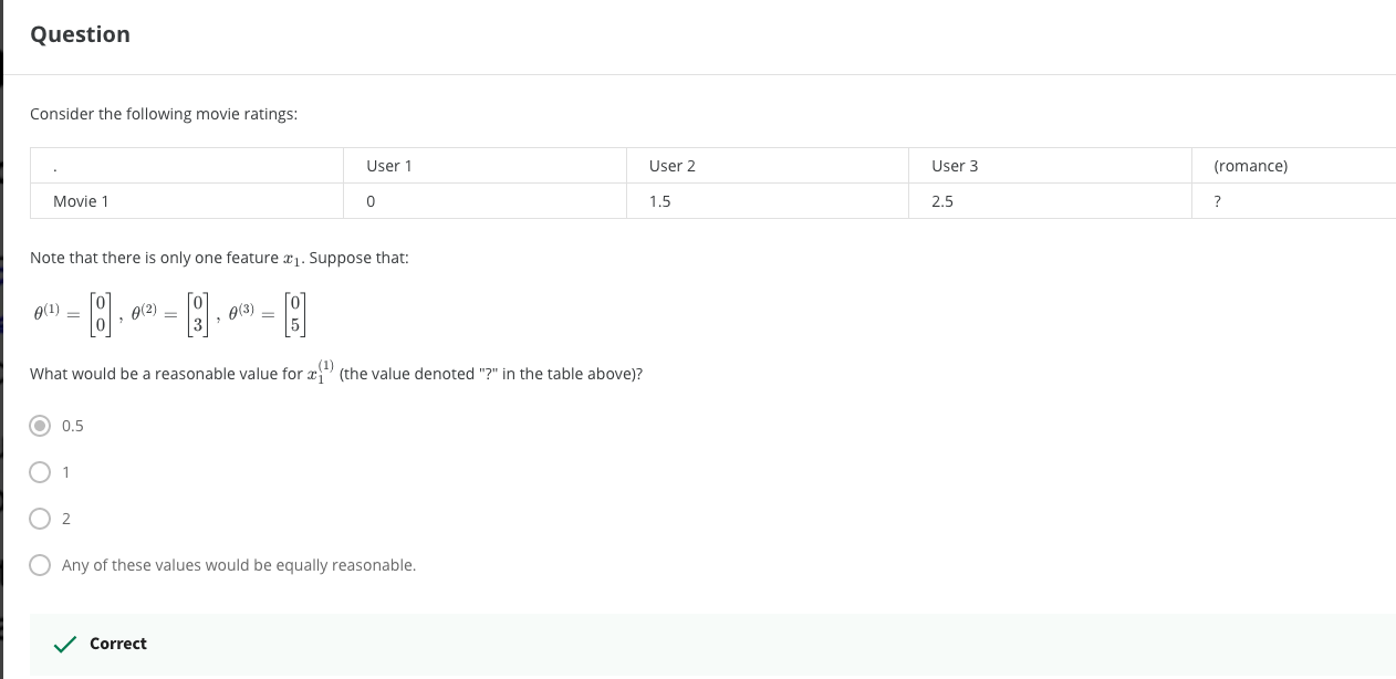
Optimization function:

Collaborative filtering

θ And x, knowing one, can get another, which becomes the question of chicken or egg first.

You can do this: guess some first θ， Calculate X; Use this x to calculate θ； Cycle

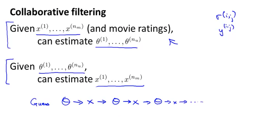
All users are contributing to a better model, so it is called collaborative filtering.

Collaborative filtering objective function and optimization at the same time θ And x, don't really alternate:

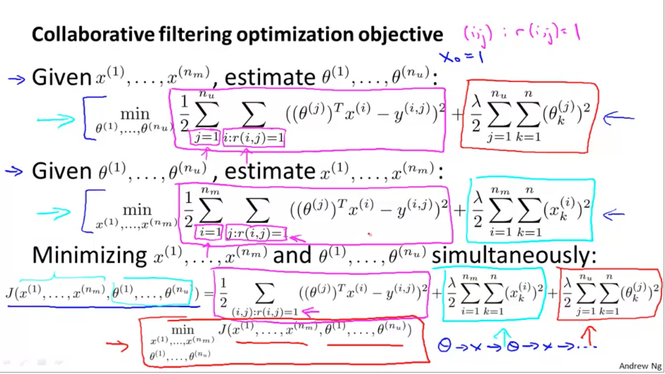
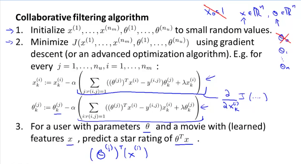
Collaborative filtering algorithm:

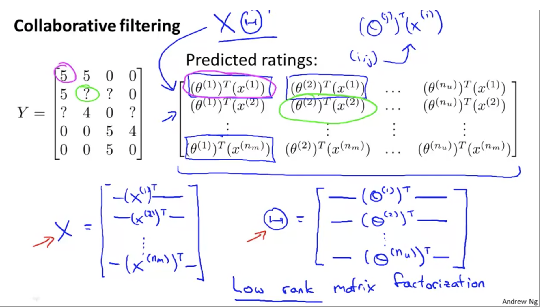
Vectorization: Low Rank Matrix Factorization

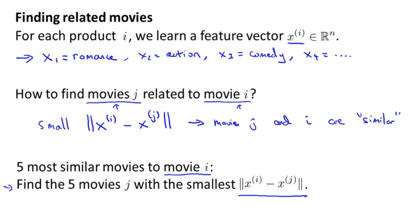
How to find relevant movies

If the difference between characteristic matrices x is small, it is more similar.

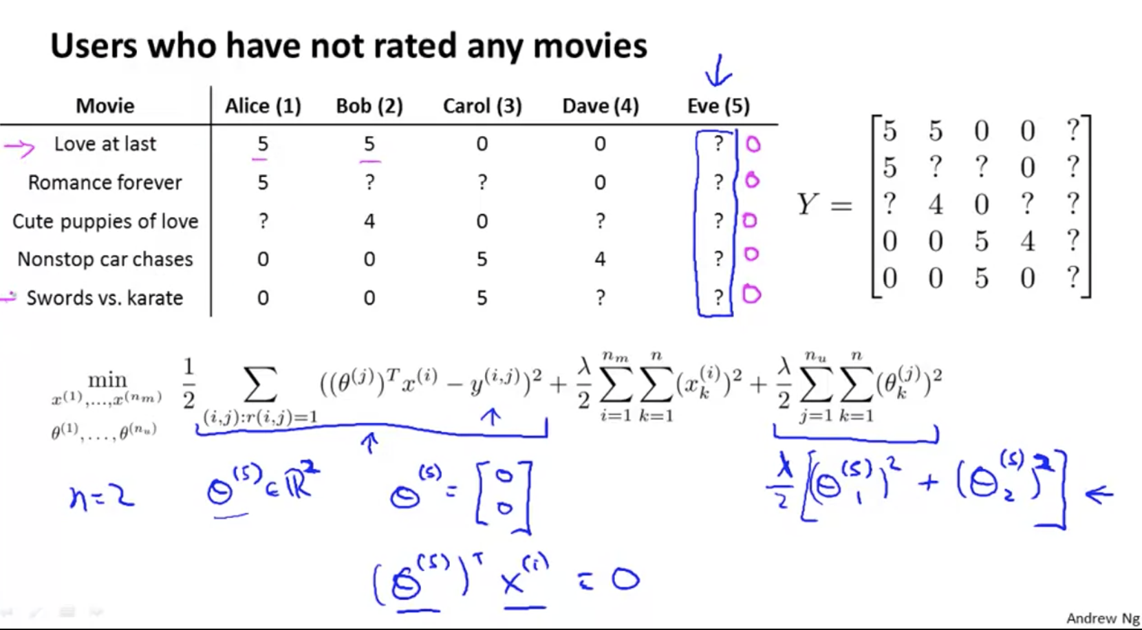
mean normalization

Problem: for Eve, she evaluates any movie, and finally calculates that her score is 0, so she can't recommend movies for her.

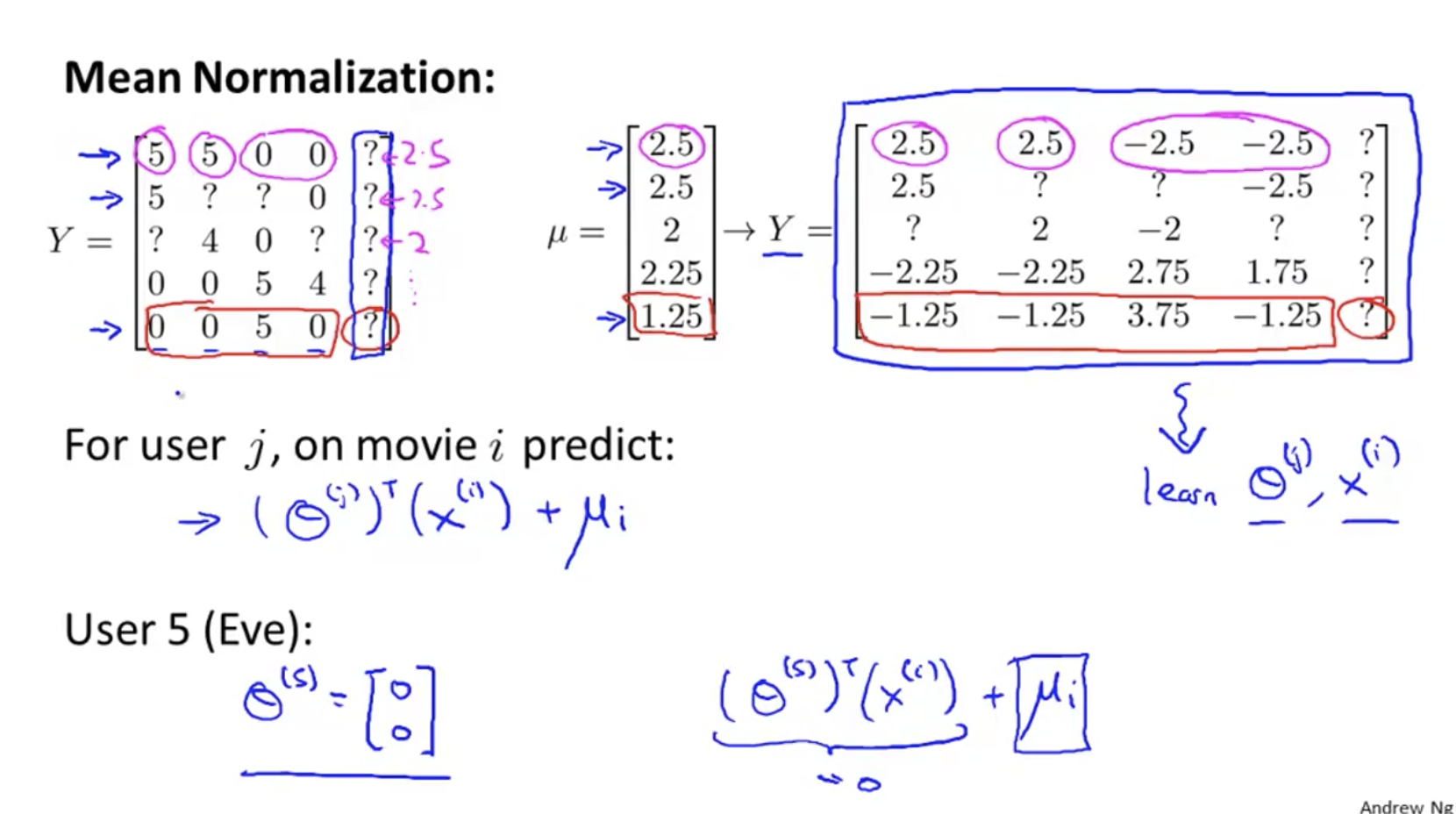
Mean normalization:
For each line, subtract the average of the line μ i；
Learn θ And x;
Result add back μ i is the prediction result.

In fact, Eve's score is predicted by the average value.

task

Using Matlab 2015b, the calculation matrix vector cannot be implicitly extended, and an error will be reported:

>> X - mu'
Error using  - 
Matrix dimensions must agree.

Solution, use bsxfun:

bsxfun(@minus, X, mu')

estimateGaussian.m

function [mu sigma2] = estimateGaussian(X)
%ESTIMATEGAUSSIAN This function estimates the parameters of a 
%Gaussian distribution using the data in X
%   [mu sigma2] = estimateGaussian(X), 
%   The input X is the dataset with each n-dimensional data point in one row
%   The output is an n-dimensional vector mu, the mean of the data set
%   and the variances sigma^2, an n x 1 vector
% 

% Useful variables
[m, n] = size(X);

% You should return these values correctly
mu = zeros(n, 1);
sigma2 = zeros(n, 1);

% ====================== YOUR CODE HERE ======================
% Instructions: Compute the mean of the data and the variances
%               In particular, mu(i) should contain the mean of
%               the data for the i-th feature and sigma2(i)
%               should contain variance of the i-th feature.
%
mu = sum(X)' ./ m;
sigma2 = sum(bsxfun(@minus, X, mu') .^ 2)' ./ m;
% =============================================================
end

selectThreshold.m

function [bestEpsilon bestF1] = selectThreshold(yval, pval)
%SELECTTHRESHOLD Find the best threshold (epsilon) to use for selecting
%outliers
%   [bestEpsilon bestF1] = SELECTTHRESHOLD(yval, pval) finds the best
%   threshold to use for selecting outliers based on the results from a
%   validation set (pval) and the ground truth (yval).
%

bestEpsilon = 0;
bestF1 = 0;
F1 = 0;

stepsize = (max(pval) - min(pval)) / 1000;

    
for epsilon = min(pval):stepsize:max(pval),
    
    % ====================== YOUR CODE HERE ======================
    % Instructions: Compute the F1 score of choosing epsilon as the
    %               threshold and place the value in F1. The code at the
    %               end of the loop will compare the F1 score for this
    %               choice of epsilon and set it to be the best epsilon if
    %               it is better than the current choice of epsilon.
    %               
    % Note: You can use predictions = (pval < epsilon) to get a binary vector
    %       of 0's and 1's of the outlier predictions
    tp = sum(yval==1 & pval < epsilon);
    fp = sum(yval==1 & pval >= epsilon);
    fn = sum(yval==0 & pval < epsilon);
    prec = tp/(tp+fp);
    rec = tp/(tp+fn);
    F1 = 2 * prec * rec / (prec + rec);
    if F1 > bestF1,
        bestF1 = F1;
        bestEpsilon = epsilon;
    end
end
    % =============================================================
end

The effect is as follows:

cofiCostFunc.m

function [J, grad] = cofiCostFunc(params, Y, R, num_users, num_movies, ...
                                  num_features, lambda)
%COFICOSTFUNC Collaborative filtering cost function
%   [J, grad] = COFICOSTFUNC(params, Y, R, num_users, num_movies, ...
%   num_features, lambda) returns the cost and gradient for the
%   collaborative filtering problem.
%

% Unfold the U and W matrices from params
X = reshape(params(1:num_movies*num_features), num_movies, num_features);
Theta = reshape(params(num_movies*num_features+1:end), ...
                num_users, num_features);

            
% You need to return the following values correctly
J = 0;
X_grad = zeros(size(X));
Theta_grad = zeros(size(Theta));

% ====================== YOUR CODE HERE ======================
% Instructions: Compute the cost function and gradient for collaborative
%               filtering. Concretely, you should first implement the cost
%               function (without regularization) and make sure it is
%               matches our costs. After that, you should implement the 
%               gradient and use the checkCostFunction routine to check
%               that the gradient is correct. Finally, you should implement
%               regularization.
%
% Notes: X - num_movies  x num_features matrix of movie features
%        Theta - num_users  x num_features matrix of user features
%        Y - num_movies x num_users matrix of user ratings of movies
%        R - num_movies x num_users matrix, where R(i, j) = 1 if the 
%            i-th movie was rated by the j-th user
%
% You should set the following variables correctly:
%
%        X_grad - num_movies x num_features matrix, containing the 
%                 partial derivatives w.r.t. to each element of X
%        Theta_grad - num_users x num_features matrix, containing the 
%                     partial derivatives w.r.t. to each element of Theta
%
J = sum(sum(((X * Theta' - Y) .* R) .^ 2)) ./ 2 + lambda .* sum(sum(Theta.^2)) ./ 2 + lambda .* sum(sum(X.^2)) ./ 2;
X_grad = (X * Theta' - Y) .* R * Theta + lambda .* X;
Theta_grad = ((X * Theta' - Y) .* R)' * X +  + lambda .* Theta;


% =============================================================

grad = [X_grad(:); Theta_grad(:)];

end