Latest features of Cartopy 0.20

Background introduction

Cartopy is a map mapping package developed by the Met Office, which realizes most of the functions of Basemap and makes use of the powerful proj 4. NumPy and Shapely libraries, and a programming interface is built on Matplotlib to create and publish quality maps, and conduct geospatial data processing and spatial data analysis, which is very useful for the majors of cartography, GIS and atmospheric science.

Although,

• The installation of Cartopy is complex. It is recommended to use conda install cartopy for installation, but many students may give up qaq from getting started because of installation.
• The function of the lower version of Cartopy (0.18 and below) is still relatively limited, and the projection of non equal longitude and latitude cannot be marked.

But,

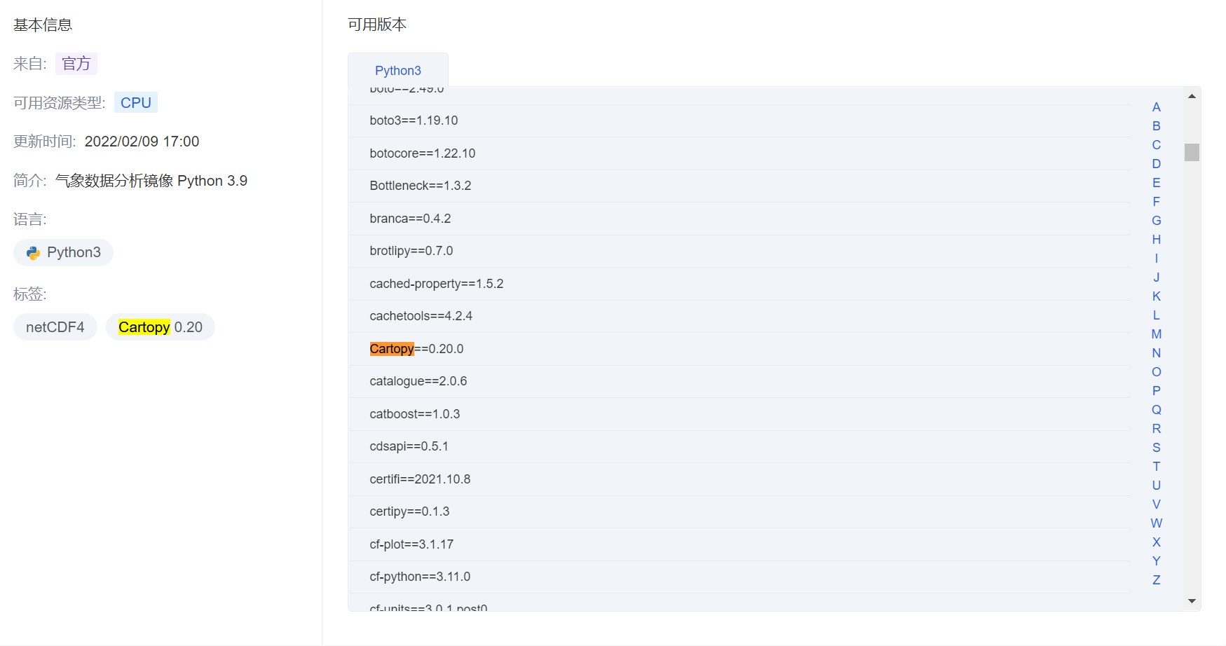
• ModelWhale provides meteorological data analysis image , it eliminates the trouble of environment configuration and module installation, and provides common Python modules for irregular maintenance and update
• The latest is based on Python 3 Version 9 image contains Cartopy 0.20 module, which integrates many new functions and is more stable and friendly
  

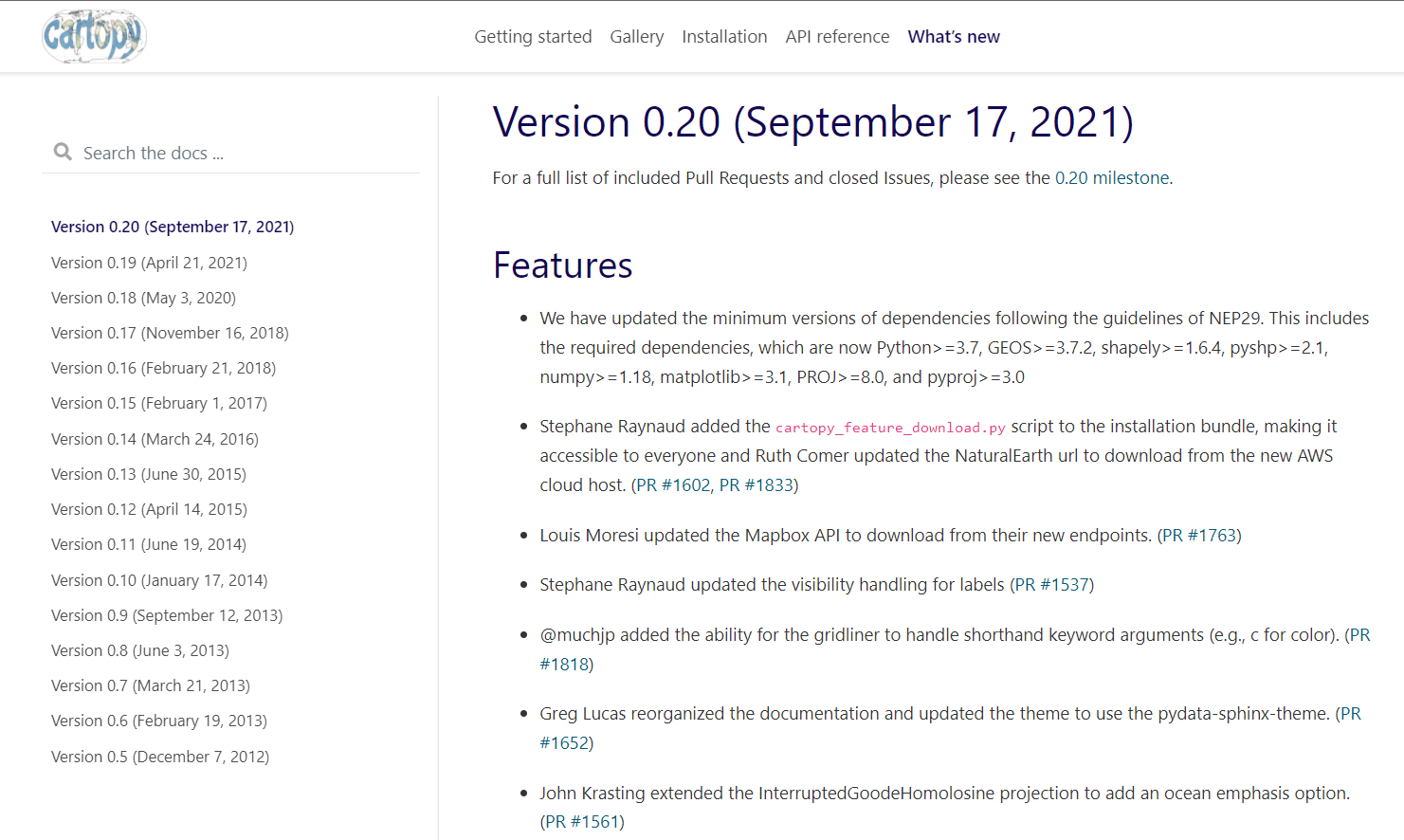
Introduction to new functions

website: https://scitools.org.uk/cartopy/docs/latest/whatsnew/v0.20.html

New function display

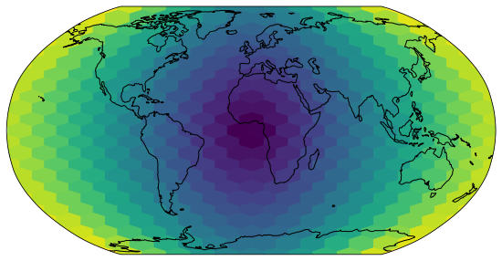
1. Support Hexagon chart (Hexbin)

fig = plt.figure(figsize=(10, 5))
ax = plt.axes(projection=ccrs.Robinson())
ax.coastlines()

x, y = np.meshgrid(np.arange(-179, 181), np.arange(-90, 91))
data = np.sqrt(x**2 + y**2)
ax.hexbin(x.flatten(), y.flatten(), C=data.flatten(),
          gridsize=20, transform=ccrs.PlateCarree())
plt.show()

2. Goode segmented projection is introduced

fig = plt.figure(figsize=(10, 5))
proj = ccrs.InterruptedGoodeHomolosine(central_longitude=-160,emphasis='ocean')
ax = plt.axes(projection=proj)
ax.stock_img()
plt.show()

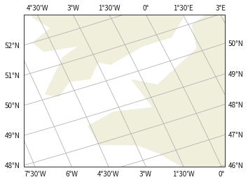
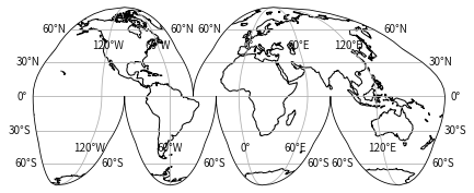
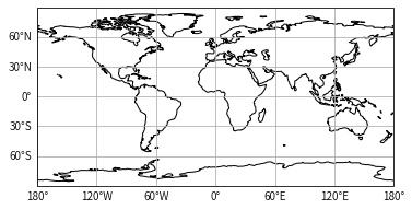
3. The problem of latitude and longitude labeling under different projections is solved

rotated_crs = ccrs.RotatedPole(pole_longitude=120.0, pole_latitude=70.0)
ax0 = plt.axes(projection=rotated_crs)
ax0.set_extent([-6, 1, 47.5, 51.5], crs=ccrs.PlateCarree())
ax0.add_feature(cfeature.LAND.with_scale('110m'))
ax0.gridlines(draw_labels=True, dms=True, x_inline=False, y_inline=False)

plt.figure(figsize=(6.9228, 3))
ax1 = plt.axes(projection=ccrs.InterruptedGoodeHomolosine())
ax1.coastlines(resolution='110m')
ax1.gridlines(draw_labels=True)

plt.figure(figsize=(7, 3))
ax2 = plt.axes(projection=ccrs.PlateCarree())
ax2.coastlines(resolution='110m')
gl = ax2.gridlines(draw_labels=True)
gl.top_labels = False
gl.right_labels = False
plt.show()

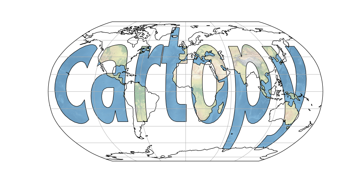
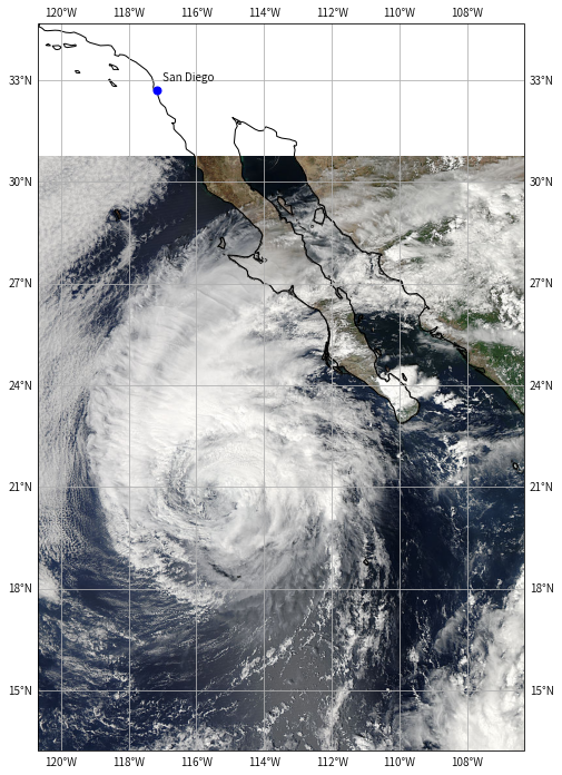
4. Project the image

fig = plt.figure(figsize=(8, 12))
# !wget https://lance-modis.eosdis.nasa.gov/imagery/gallery/2012270-0926/Miriam.A2012270.2050.2km.jpg
fname = '/home/mw/project/Miriam.A2012270.2050.2km.jpg'
img_extent = (-120.67660000000001, -106.32104523100001, 13.2301484511245, 30.766899999999502)
img = plt.imread(fname)
ax = plt.axes(projection=ccrs.PlateCarree())
ax.set_xmargin(0.05)
ax.set_ymargin(0.10)
ax.imshow(img, origin='upper', extent=img_extent, transform=ccrs.PlateCarree())
ax.coastlines(resolution='50m', color='black', linewidth=1)
ax.gridlines(draw_labels=True, dms=True, x_inline=False, y_inline=False)
ax.plot(-117.1625, 32.715, 'bo', markersize=7, transform=ccrs.Geodetic())
ax.text(-117, 33, 'San Diego', transform=ccrs.Geodetic())
plt.show()

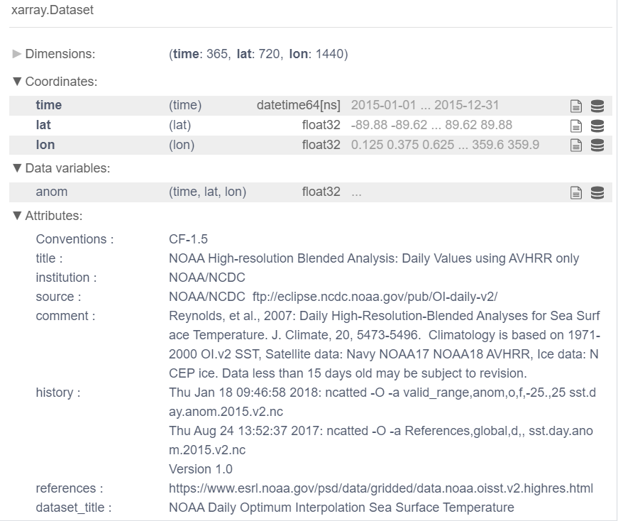
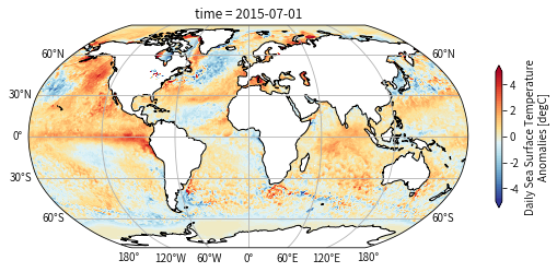
5. Perfect compatibility with xarray

ds = xr.open_dataset('/home/mw/input/OISSTV27010/anom/sst.day.anom.2015.nc')
ds

ssta = ds.anom.sel(time='2015-07-01', method='nearest')
fig = plt.figure(figsize=(9,6))
ax = plt.axes(projection=ccrs.Robinson())
ax.coastlines()
gl = ax.gridlines(draw_labels=True, dms=True, x_inline=False, y_inline=False)
gl.top_labels = False
gl.right_labels = False
ssta.plot(ax=ax, transform=ccrs.PlateCarree(),
          vmin=-5, vmax=5, cmap=cmaps.cmp_b2r,
          cbar_kwargs={'shrink': 0.4})
plt.show()

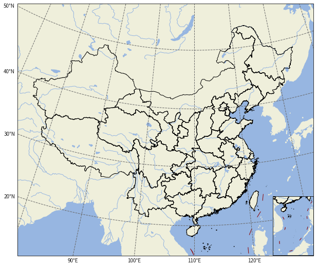
6. Draw the territory of China of Lambert projection

Standard map services: http://211.159.153.75/

The standard map is prepared according to the drawing standards of national boundaries between China and other countries in the world. It can be used for news publicity, illustrations of books, periodicals and newspapers, background map of advertising display, base map of handicraft design, etc. it can also be used as the reference base map for preparing public version map. The public can browse and download the standard map for free. When using the standard map directly, the drawing review number needs to be marked.

# Set projection
proj = ccrs.LambertConformal(central_longitude=110, central_latitude=90,standard_parallels=(25, 47))

# Create Legend
fig = plt.figure(figsize=(10, 8),frameon=True)
ax = fig.add_axes([0.08, 0.05, 0.8, 0.94], projection=proj)
ax.set_extent([80, 130, 15, 55],crs=ccrs.PlateCarree())
ax.tick_params(labelsize=15)

# Add base geographic layer
ax.add_feature(cfeature.OCEAN.with_scale('50m'))
ax.add_feature(cfeature.LAND.with_scale('50m'))
ax.add_feature(cfeature.RIVERS.with_scale('50m'))
ax.add_feature(cfeature.LAKES.with_scale('50m'))

# Add provincial boundaries and nine polylines
province = shpreader.Reader('/home/mw/input/china_shp3798/province.shp')
nineline = shpreader.Reader('/home/mw/input/china_shp3798/nine_line.shp')
ax.add_geometries(province.geometries(), crs=ccrs.PlateCarree(), edgecolor='k',facecolor='none')
ax.add_geometries(nineline.geometries(), crs=ccrs.PlateCarree(), color='#8B0000')


# Mark latitude and longitude
gl = ax.gridlines(draw_labels=True, x_inline=False, y_inline=False, dms=True,
                  xlocs=np.arange(50,170,10), ylocs=np.arange(0,60,10), 
                  linestyle='--', lw=1, rotate_labels=False,
                  color='dimgrey', crs=ccrs.PlateCarree())
gl.top_labels = False
gl.right_labels = False

# Add South China Sea drawings
sub_ax = fig.add_axes([0.75, 0.095, 0.15, 0.2],
                      projection=ccrs.LambertConformal(central_latitude=90,
                                                       central_longitude=110))
# Add base geographic layer
sub_ax.add_feature(cfeature.OCEAN.with_scale('50m'))
sub_ax.add_feature(cfeature.LAND.with_scale('50m'))
sub_ax.add_feature(cfeature.RIVERS.with_scale('50m'))
sub_ax.add_feature(cfeature.LAKES.with_scale('50m'))

# Add provincial boundaries and nine polylines
sub_ax.set_extent([106, 120, 2, 24],crs=ccrs.PlateCarree())
sub_ax.add_geometries(province.geometries(), crs=ccrs.PlateCarree(), edgecolor='k',facecolor='none')
sub_ax.add_geometries(nineline.geometries(), crs=ccrs.PlateCarree(), color='#8B0000')

plt.show()