I. ElasticSearch document score_ Underlying principle of score calculation
1.1 step 1: boolean model
According to the user's query conditions, the doc containing the specified term is filtered out first
query "hello world" -->  hello / world / hello & world

bool --> must/must not/should --> filter --> contain / Not included / May contain

doc --> No score --> Positive or negative true or false --> In order to reduce the cost to be calculated later doc Quantity and performance improvement
1.2 the second step is the relevance score algorithm
In short, it is to calculate the association matching degree between the text in an index and the search text
Elasticsearch uses the term frequency/inverse document frequency algorithm (slash represents the division between the two), which is abbreviated as TF/IDF algorithm (frequency: frequency, inverse: inversion)
Term frequency: how many times each term in the search text appears in the field text. The more it appears, the more relevant it is
For example, search request: hello world

doc1: hello you, and world is very good

doc2: hello, how are you

doc1 There are 7 words in total, and two of them are consistent; doc2 There are four words in the, and one matches
Inverse document frequency: how many times each term in the search text appears in all documents in the whole index, and the more times it appears, the less relevant it will be (it can be understood that this word appears too many times, indicating that it may be a general word with little meaning, such as "de", "ah", "Le", etc.)
Search request: hello world

doc1: hello, tuling is very good

doc2: hi world, how are you

doc1 In, there are 5 words in total, one of which is consistent; doc2 There are five words in the book, and one of them matches
For example, there are 10000 documents in the index, and the word hello appears 1000 times in all documents; The word world appears 100 times in all documents; According to the above algorithm, doc2 scores higher
Field length norm: field length. The longer the field, the weaker the correlation
Search request: hello world
doc1: { "title": "hello article", "content": "...... N Words" }

doc2: { "title": "my article", "content": "...... N A word, hi world" }
hello world appears the same number of times in the whole index
doc1 is more relevant (higher score) because the title field is shorter (there are only two words in the title, one of which is a flat match)
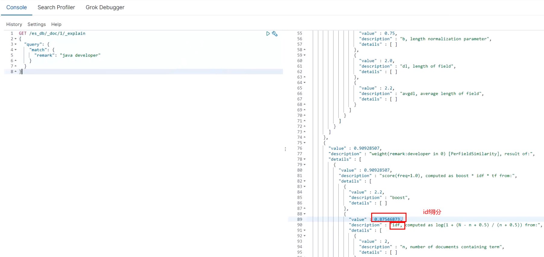
Analyze the information on a document_ How is score calculated
# _ explain to view the detailed score
GET /es_db/_doc/1/_explain
{
  "query": {
    "match": {
      "remark": "java developer"
    }
  }
}
vector space model
Total score of multiple term s to one doc
query vector
The search keyword hello world -- > es will calculate a query vector and query vector according to the score of hello world in all doc s
The term hello gives a score of 3 based on all doc s
The world term gives a score of 6 based on all doc s
So the score of query vector -- query vector is: [3, 6]
doc vector
Three doc s, one containing Hello, one containing world, one containing hello and world
The three doc s are as follows
doc1: including hello -- > [3, 0]
doc2: contains world -- > [0, 6]
doc3: including Hello, world -- > [3, 6]
Each doc will be given a score calculated for each term. hello has a score, the world has a score, and then take the scores of all terms to form a doc vector
Draw in a diagram, take the radian of each doc vector to query vector, and give the total score of each doc to multiple term s
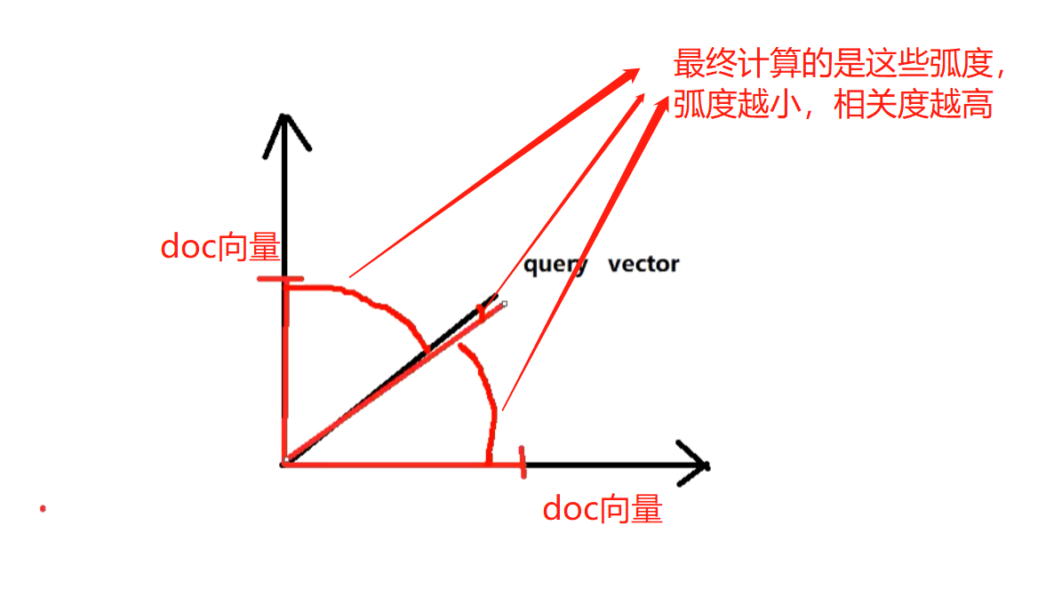
Each doc vector calculates the radian of the query vector, and finally gives the total score of a doc relative to multiple term s in the query based on this radian
The greater the radian, the lower the score at the end of the month; The smaller the radian, the higher the score
If there are multiple term s, they are calculated by linear algebra and cannot be represented by graph

Binary word splitter workflow
2.1 segmentation and normalization
Give you a sentence, and then split it into single words one by one. At the same time, normalize each word (tense conversion, singular and plural conversion, remove useless words / words (such as "de", "ah" and "Le")
recall: when searching, increase the number of results that can be searched
The main steps are as follows
character filter: Before word segmentation of a text, preprocess it first. For example, the most common is filtering html Label(<span>hello<span> --> hello),& --> and(I&you --> I and you),Or convert special characters, etc

tokenizer: Participle, hello you and me --> hello, you, and, me

token filter: lowercase(Turn lowercase),stop word,synonymom(Dealing with synonyms), liked --> like,Tom --> tom,a/the/an --> Kill useless words, small --> little(Synonym conversion)
A word splitter is very important. It processes a paragraph of text in various ways, and the final processed result will be used to establish an inverted index
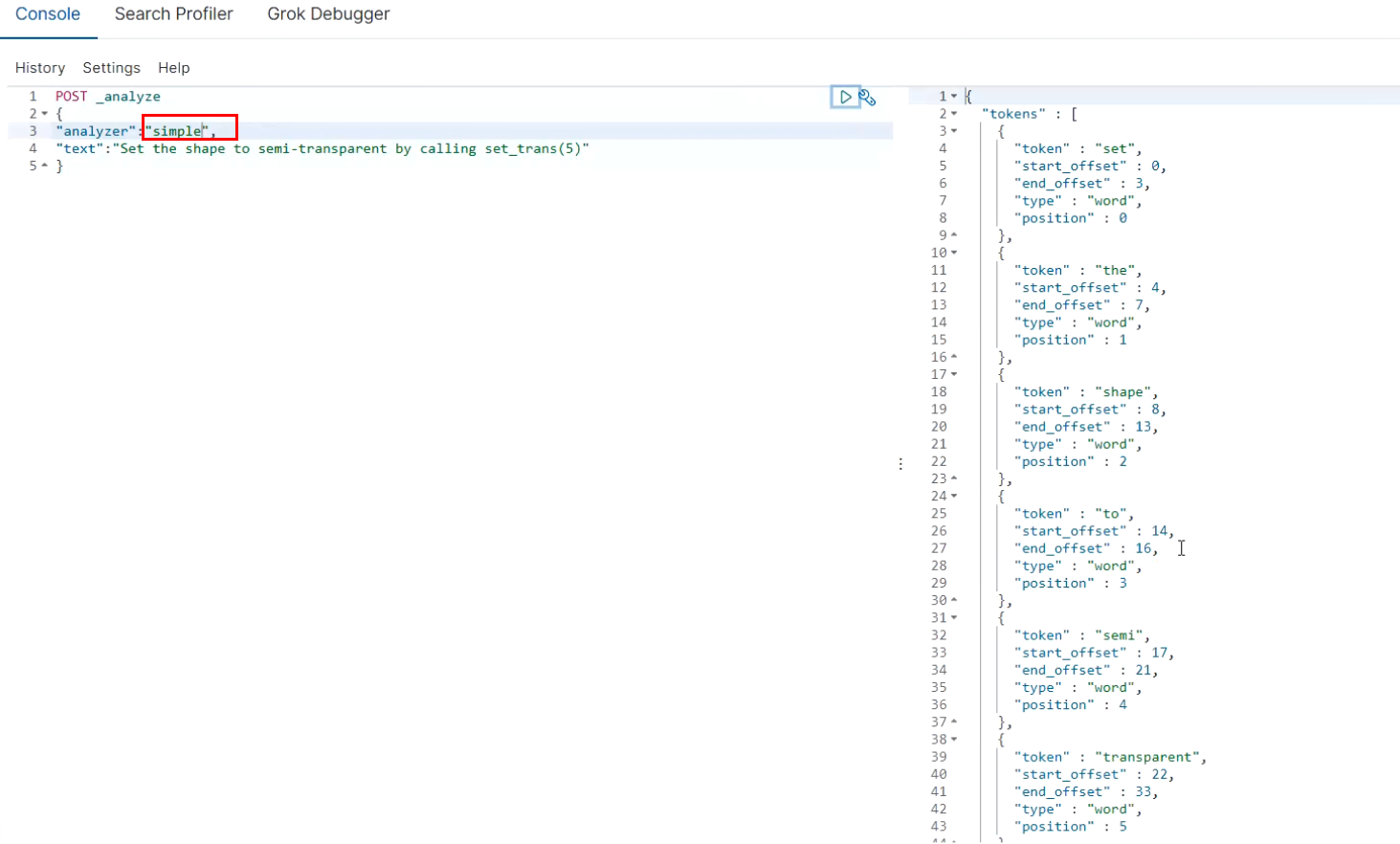
2.2 introduction of built-in word splitter
Set the shape to semi-transparent by calling set_trans(5)

Several built-in word splitters:

standard analyzer: set, the, shape, to, semi, transparent, by, calling, set_trans, 5(The default is standard)

simple analyzer: set, the, shape, to, semi, transparent, by, calling, set, trans

whitespace(Space segmentation) analyzer: Set, the, shape, to, semi-transparent, by, calling, set_trans(5)

stop analyzer:Remove stop words, such as a the it Wait, get rid of it

Test:
POST _analyze
{
"analyzer":"standard",
"text":"Set the shape to semi-transparent by calling set_trans(5)"
}
2.3 custom word splitter
2.3.1 default word splitter
standard
standard tokenizer: segmentation based on word boundaries
standard token filter: do nothing
lowercase token filter: converts all letters to lowercase
stop token filer (disabled by default): remove stop words, such as a the it, etc
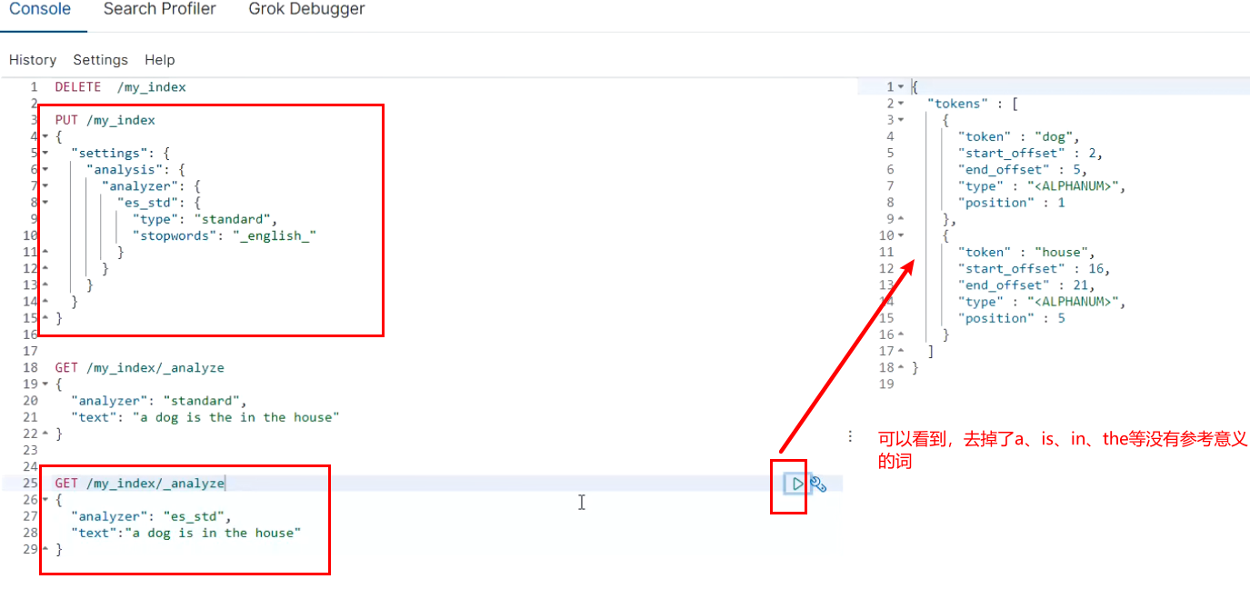
2.3.2 modify the setting of word splitter
Enable the english stop word token filter
PUT /my_index
{
  "settings": {
    "analysis": {
      "analyzer": {
        "es_std": {
          "type": "standard",
          "stopwords": "_english_"
        }
      }
    }
  }
}

GET /my_index/_analyze
{
  "analyzer": "es_std",
  "text":"a dog is in the house"
}
3,Customize your own word splitter

PUT /my_index
{
"settings": {
"analysis": {
"char_filter": {
#Just take the name yourself
"&_to_and": {
"type": "mapping",
#Replace the symbol & with and, and separate multiple conditions with commas
"mappings": ["&=> and"]
}
},
"filter": {
#Name yourself
"my_stopwords": {
"type": "stop",
#Stop the words the and a
"stopwords": ["the", "a"]
}
},
"analyzer": {
"my_analyzer": {
#This value cannot be written casually. If it is a custom word splitter, only custom can be written here
"type": "custom",
#html_strip: tags in HTML are automatically filtered out (such as a tag)
#&_ to_ And: the name of the custom word splitter above
"char_filter": ["html_strip", "&_to_and"],
#Custom word splitter based on standard word splitter
"tokenizer": "standard",
# Lowercase: automatically convert uppercase to lowercase
# my_stopwords: the name of the custom word splitter above
"filter": ["lowercase", "my_stopwords"]
}
}
}
}
}

GET /my_index/_analyze
{
"text": "tom&jerry are a friend in the house, <a>, HAHA!!",
"analyzer": "my_analyzer"
}

PUT /my_index/_mapping/my_type
{
"properties": {
"content": {
"type": "text",
"analyzer": "my_analyzer"
}
}
}
2.4 ik word splitter details
Directory: ik / config / plugins
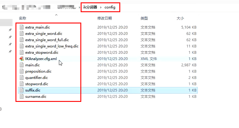
IKAnalyzer.cfg.xml: used to configure custom thesaurus
main.dic: ik's native built-in Chinese Thesaurus has a total of more than 270000 words. As long as these words are divided together
quantifier.dic: put some words related to units
suffix.dic: put some suffixes
surname.dic: Chinese surname
stopword.dic: English stop word
The two most important configuration files of ik native
main.dic: contains native Chinese words, which will be segmented according to the words in it
stopword.dic: contains English stop words
stopword
a the and at but
Generally, like stop words, they will be directly killed during word segmentation and will not be established in the inverted index
2.4 IK word splitter custom Thesaurus
(1) Build your own Thesaurus: every year, some special popular words will emerge, such as net red, blue thin mushroom, shouting wheat and ghost livestock. These words are generally not in ik's original dictionary. You need to supplement your own latest words and go to ik's Thesaurus
Open ikanalyzer.com in the conf folder under ik word splitter cfg. XML: add ext_dict, new directory and file: Custom / mydict dic,mydict. Write your own hot words in DIC
Add your own words, and then restart es to take effect
Create your own vocabulary file:
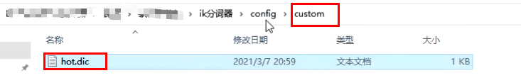
Write one word on each line:
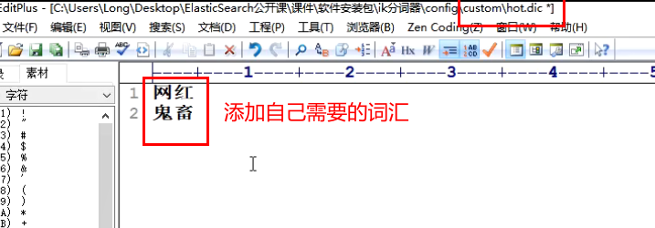
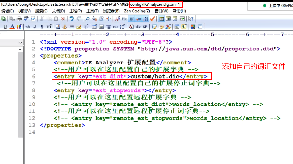
Then at ikanalyzer cfg. Add your own vocabulary file address in XML
(2) Build a stop thesaurus by ourselves (there is a specific configuration in the figure above): for example, we may not want to build an index for others to search
custom/ext_stopword.dic, which has commonly used Chinese stop words, can supplement its own stop words, and then restart es
IK word splitter source code download: https://github.com/medcl/elasticsearch-analysis-ik/tree
2.5 IK hot update
Every time in Chapter 2.4, new words are added manually in the extended Dictionary of es, which is very boring
- After each addition, you have to restart es to take effect. It's very troublesome
- es is distributed. There may be hundreds of nodes. You can't modify one node at a time
es does not stop. We can add new words in an external place directly, and these new words will be hot loaded in es immediately
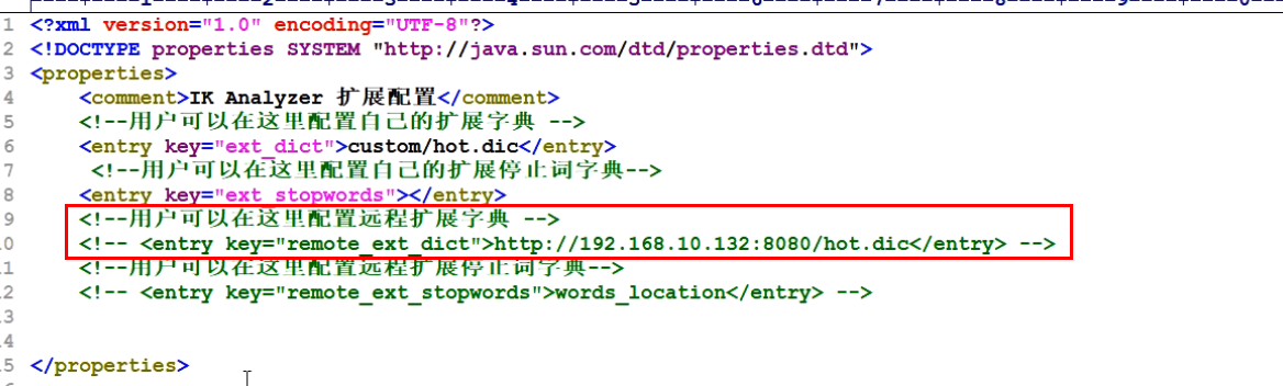
IKAnalyzer. cfg. The XML file is as follows:
<properties>
	<comment>IK Analyzer Extended configuration</comment>
	<!--Users can configure their own extended dictionary here -->
	<entry key="ext_dict">location</entry>
	 <!--Users can configure their own extended stop word dictionary here-->
	<entry key="ext_stopwords">location</entry>
	<!--Users can configure the remote extension dictionary here -->
	<entry key="remote_ext_dict">words_location</entry>
	<!--Users can configure the remote extended stop word dictionary here-->
	<entry key="remote_ext_stopwords">words_location</entry>
</properties>
Remote mode I
Not recommended. Sometimes there are bug s
For example, change this way (add a Tomcat deployed in the remote tomcat, with the configuration file hot.dic inside):
Remote mode II
You need to change the source code of IK word splitter. Download the source code of IK word splitter: https://github.com/medcl/elasticsearch-analysis-ik/tree
Principle of modifying ik source code: use ik source code to connect to the local mysql database, and set two tables in the library. One is to save the old vocabulary before ik, and the other is to save the new hot vocabulary. In the future, you only need to change the data in the hot list in the database;
The specific steps to change the source code will be described in the blog in the next chapter
Three Highlights
In search, it is often necessary to highlight search keywords. Highlighting also has its common parameters. In this case, some common parameters are introduced.
Now search for the document containing "Volkswagen" in the remark field of the cars index. The "XX keyword" is highlighted. html tag is used for the highlighting effect, and the font is set to red. If the remark data is too long, only the first 20 characters are displayed.
PUT /news_website
{
"mappings": {
"properties": {
"title": {
"type": "text",
"analyzer": "ik_max_word"
},
"content": {
"type": "text",
"analyzer": "ik_max_word"
}
}
}
}
# The code for establishing the index library above can also be written in the following way
PUT /news_website
{
"settings" : {
"index" : {
"analysis.analyzer.default.type": "ik_max_word"
}
}
}
# Insert a piece of data
PUT /news_website/_doc/1
{
"title": "This is the first article I wrote",
"content": "Hello everyone, this is the first article I wrote. I especially like this article portal!!!"
}
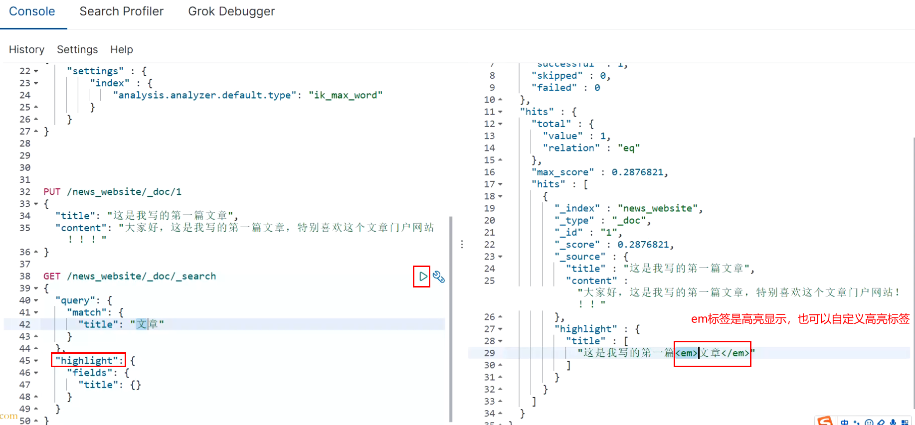
# query
GET /news_website/_doc/_search
{
"query": {
"match": {
"title": "article"
}
},
# Highlighted fields
"highlight": {
"fields": {
"title": {}
}
}
}
# Query results
{
"took" : 458,
"timed_out" : false,
"_shards" : {
"total" : 1,
"successful" : 1,
"skipped" : 0,
"failed" : 0
},
"hits" : {
"total" : {
"value" : 1,
"relation" : "eq"
},
"max_score" : 0.2876821,
"hits" : [
{
"_index" : "news_website",
"_type" : "_doc",
"_id" : "1",
"_score" : 0.2876821,
"_source" : {
"title" : "My first article",
"content" : "Hello everyone, this is the first article I wrote. I especially like this article portal!!!"
},
"highlight" : {
"title" : [
"My first article<em>article</em>"
]
}
}
]
}
}
<em></em>Performance, will turn red, so your designated field If the search term is included, it will be in that field In the text of, highlight the search term in red
GET /news_website/_doc/_search
{
  "query": {
    "bool": {
      "should": [
        {
          "match": {
            "title": "article"
          }
        },
        {
          "match": {
            "content": "article"
          }
        }
      ]
    }
  },
  "highlight": {
    "fields": {
      "title": {},
      "content": {}
    }
  }
}

highlight Medium field,Must follow query Medium field One by one aligned

2,frequently-used highlight Introduction (three kinds)

First: plain highlight(Default), based on lucene highlight

Second: posting highlight,index_options=offsets

(1)posting highlight Performance ratio plain highlight It should be higher because there is no need to re segment the highlighted text
(2)posting highlight Less disk consumption


DELETE news_website
PUT /news_website
{
  "mappings": {
      "properties": {
        "title": {
          "type": "text",
          "analyzer": "ik_max_word"
        },
        "content": {
          "type": "text",
          "analyzer": "ik_max_word",
          # Set highlight mode
          "index_options": "offsets"
        }
      }
  }
}

PUT /news_website/_doc/1
{
  "title": "My first article",
  "content": "Hello everyone, this is the first article I wrote. I especially like this article portal!!!"
}

GET /news_website/_doc/_search
{
  "query": {
    "match": {
      "content": "article"
    }
  },
  "highlight": {
    "fields": {
      "content": {}
    }
  }
}

Third: fast vector highlight

index-time term vector Set in mapping Yes, I can use it fast verctor highlight

(1)Right big field For (greater than 1) mb),Higher performance

delete  /news_website

PUT /news_website
{
  "mappings": {
      "properties": {
        "title": {
          "type": "text",
          "analyzer": "ik_max_word"
        },
        "content": {
          "type": "text",
          "analyzer": "ik_max_word",
          "term_vector" : "with_positions_offsets"
        }
      }
  }
}

Force the use of a highlighter,For example, for open term vector of field Generally speaking, it can be used forcibly plain highlight

GET /news_website/_doc/_search
{
  "query": {
    "match": {
      "content": "article"
    }
  },
  "highlight": {
    "fields": {
      "content": {
        "type": "plain"
      }
    }
  }
}

To sum up, you can actually consider it according to your actual situation. Generally, use plain highlight That's enough. There's no need to make other additional settings
 If you have high performance requirements for highlighting, you can try to enable it posting highlight
 If field The value of is particularly large, exceeding 1 M,Then it can be used fast vector highlight

3,Set highlight html Label, default is<em>label

GET /news_website/_doc/_search
{
  "query": {
    "match": {
      "content": "article"
    }
  },
  "highlight": {
    "pre_tags": ["<span color='red'>"],
    "post_tags": ["</span>"],
    "fields": {
      "content": {
        "type": "plain"
      }
    }
  }
}

4,Highlight clip fragment Settings for

GET /_search
{
    "query" : {
        "match": { "content": "article" }
    },
    "highlight" : {
        "fields" : {
            "content" : {"fragment_size" : 150, "number_of_fragments" : 3 }
        }
    }
}

fragment_size: You one Field For example, the length is 10000, but you can't display it on the page so long... Set the to be displayed fragment The length of text judgment is 100 by default
number_of_fragments: You may be your highlight fragment The text segment has multiple segments. You can specify how many segments to display
IV. in depth of aggregation search technology
4.1 introduction to bucket and metric concepts
A bucket is a data grouping for aggregate search. For example, the sales department has employees Zhang San and Li Si, and the development department has employees Wang Wu and Zhao Liu. Then, according to the Department grouping and aggregation, the result is two buckets. There are Zhang San and Li Si in the bucket of the sales department,
There are Wang Wu and Zhao Liu in the bucket of the development department.
Metric is the statistical analysis of a bucket data. For example, in the above case, there are two employees in the development department and two employees in the sales department, which is metric.
metric has a variety of statistics, such as summation, maximum, minimum, average, etc.
Use an easy to understand SQL syntax to explain, such as: select count(*) from table group by column, then each group of data after group by column is bucket. The count(*) executed for each group is metric.
4.2 preparation of case data
PUT /cars
{
"mappings": {
"properties": {
"price": {
"type": "long"
},
"color": {
"type": "keyword"
},
"brand": {
"type": "keyword"
},
"model": {
"type": "keyword"
},
"sold_date": {
"type": "date"
},
"remark" : {
"type" : "text",
"analyzer" : "ik_max_word"
}
}
}
}
POST /cars/_bulk
{ "index": {}}
{ "price" : 258000, "color" : "golden", "brand":"public", "model" : "MAGOTAN", "sold_date" : "2021-10-28","remark" : "Volkswagen mid-range car" }
{ "index": {}}
{ "price" : 123000, "color" : "golden", "brand":"public", "model" : "Volkswagen Sagitar", "sold_date" : "2021-11-05","remark" : "Volkswagen divine vehicle" }
{ "index": {}}
{ "price" : 239800, "color" : "white", "brand":"sign", "model" : "Sign 508", "sold_date" : "2021-05-18","remark" : "Global market model of logo brand" }
{ "index": {}}
{ "price" : 148800, "color" : "white", "brand":"sign", "model" : "Sign 408", "sold_date" : "2021-07-02","remark" : "Relatively large compact car" }
{ "index": {}}
{ "price" : 1998000, "color" : "black", "brand":"public", "model" : "Volkswagen Phaeton", "sold_date" : "2021-08-19","remark" : "Volkswagen's most painful car" }
{ "index": {}}
{ "price" : 218000, "color" : "gules", "brand":"audi", "model" : "audi A4", "sold_date" : "2021-11-05","remark" : "Petty bourgeoisie model" }
{ "index": {}}
{ "price" : 489000, "color" : "black", "brand":"audi", "model" : "audi A6", "sold_date" : "2022-01-01","remark" : "For government use?" }
{ "index": {}}
{ "price" : 1899000, "color" : "black", "brand":"audi", "model" : "audi A 8", "sold_date" : "2022-02-12","remark" : "Very expensive big A6. . . " }
V. aggregation operation cases
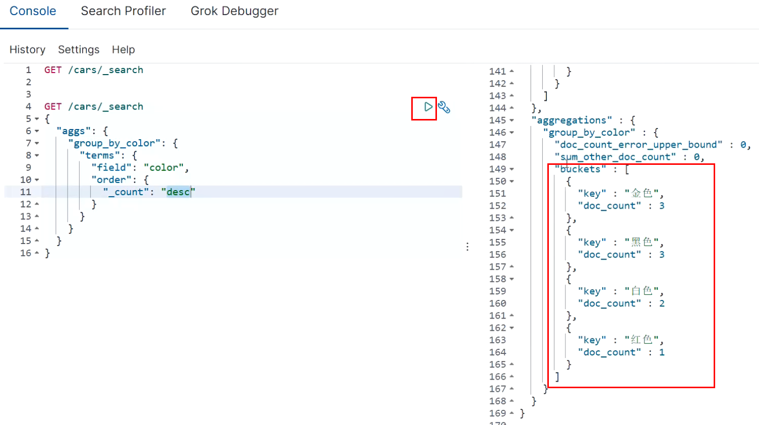
5.1 statistics of sales quantity by color group
Only aggregate grouping is performed without complex aggregate statistics. In ES, the most basic aggregation is terms, which is equivalent to count in SQL.
In ES, grouping data is sorted by default, and DOC is used_ Arrange data in descending order count. Can use_ key metadata, which implements different sorting schemes according to the grouped field data, or_ Count metadata, which implements different sorting schemes according to the grouped statistical values.
GET /cars/_search
{
# aggs stands for aggregate query
"aggs": {
# alias
"group_by_color": {
"terms": {
"field": "color",
"order": {
# _ count: the default value of the bottom layer, which means sorting by quantity
"_count": "desc"
}
}
}
}
}
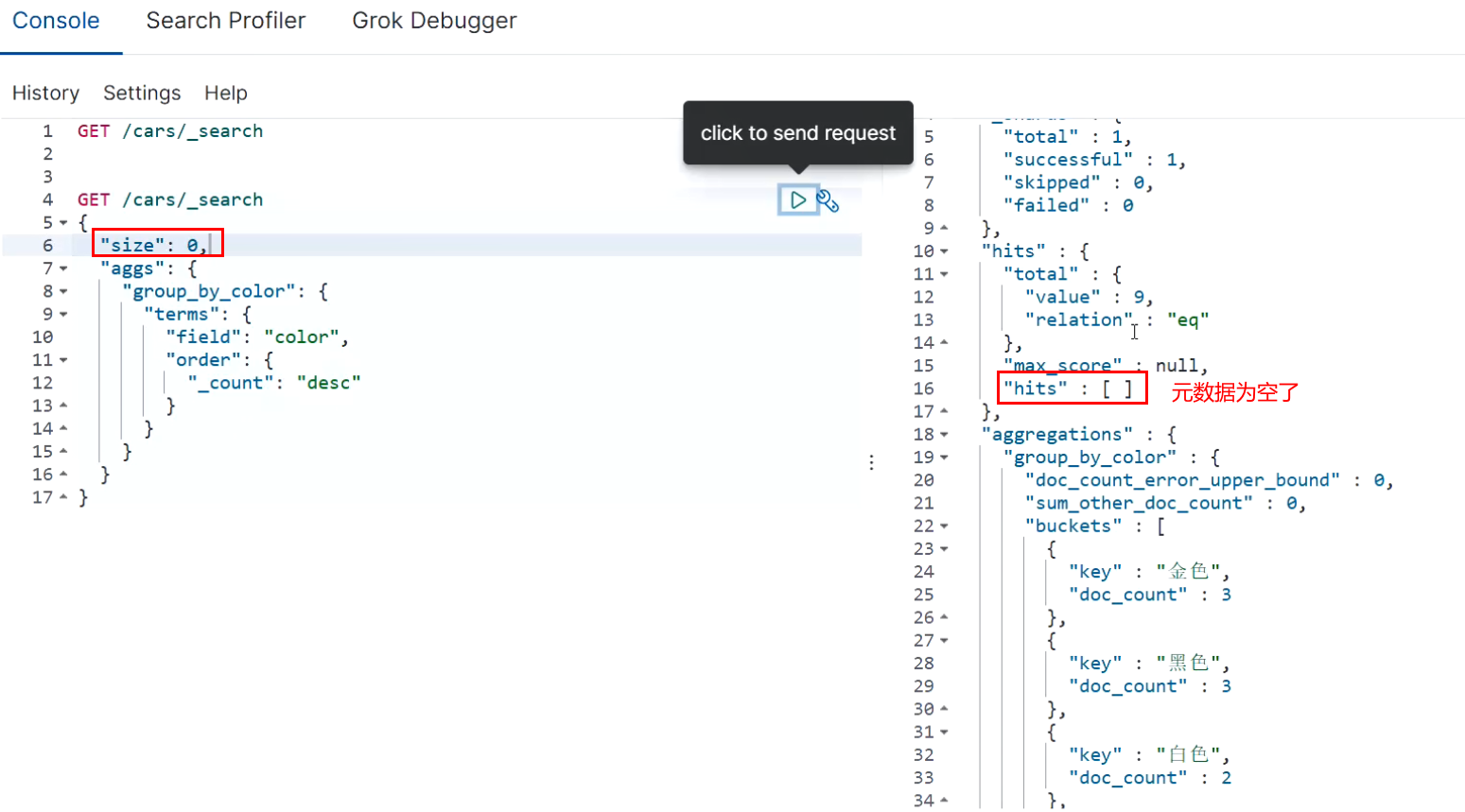
The results above contain a lot of metadata. If we don't want to see these metadata but only want to see the aggregated results, we can add the parameter edge during query
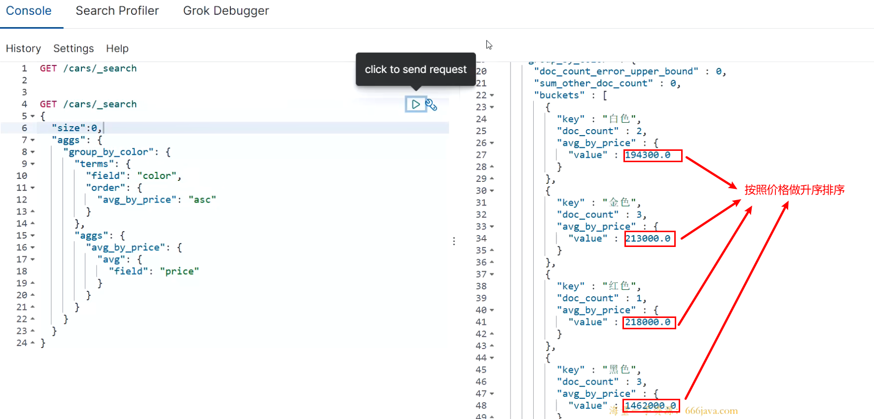
5.2 statistics of average prices of vehicles with different color s
In this case, we first perform aggregation grouping according to color. On the basis of this grouping, we perform aggregation statistics on the data in the group. The aggregation statistics of the data in the group is metric. Sorting can also be performed because there are aggregate statistics in the group and the statistics are named avg_by_price, so the sorting logic can be executed according to the field name of the aggregated statistics.
GET /cars/_search
{
"aggs": {
"group_by_color": {
"terms": {
"field": "color",
"order": {
"avg_by_price": "asc"
}
},
"aggs": {
"avg_by_price": {
"avg": {
"field": "price"
}
}
}
}
}
}
size can be set to 0, which means that the documents in ES are not returned, but only the data after ES aggregation is returned to improve the query speed. Of course, if you need these documents, you can also set them according to the actual situation
GET /cars/_search
{
"size" : 0,
"aggs": {
"group_by_color": {
"terms": {
"field": "color"
},
"aggs": {
"group_by_brand" : {
"terms": {
"field": "brand",
"order": {
"avg_by_price": "desc"
}
},
"aggs": {
"avg_by_price": {
"avg": {
"field": "price"
}
}
}
}
}
}
}
}
5.3 statistics on the average price of vehicles in different color s and brand s
First group according to color, and then group according to brand in the group. This operation can be called drill down analysis.
If there are many definitions of aggs, you will feel that the syntax format is chaotic. The aggs syntax format has a relatively fixed structure and simple definition: aggs can be nested and horizontal.
Nested definitions are called run in analysis. Define multiple tiling methods.
GET /index_name/type_name/_search
{
"aggs" : {
"Define group name (outermost layer)": {
"Grouping strategies, such as: terms,avg,sum" : {
"field" : "By which field",
"Other parameters" : ""
},
"aggs" : {
"Group name 1" : {},
"Group name 2" : {}
}
}
}
}
GET /cars/_search
{
"aggs": {
"group_by_color": {
"terms": {
"field": "color",
"order": {
"avg_by_price_color": "asc"
}
},
"aggs": {
"avg_by_price_color" : {
"avg": {
"field": "price"
}
},
"group_by_brand" : {
"terms": {
"field": "brand",
"order": {
"avg_by_price_brand": "desc"
}
},
"aggs": {
"avg_by_price_brand": {
"avg": {
"field": "price"
}
}
}
}
}
}
}
}
5.4 count the maximum and minimum prices and total prices in different color s
GET /cars/_search
{
"aggs": {
"group_by_color": {
"terms": {
"field": "color"
},
"aggs": {
"max_price": {
"max": {
"field": "price"
}
},
"min_price" : {
"min": {
"field": "price"
}
},
"sum_price" : {
"sum": {
"field": "price"
}
}
}
}
}
}
In common business, the most common types of aggregation analysis are statistical quantity, maximum, minimum, average, total, etc. It usually accounts for more than 60% of aggregation business, and even more than 85% of small projects.
5.5 make statistics on the models with the highest price among different brands of cars
After grouping, you may need to sort the data in the group and select the data with the highest ranking. Then you can use s to implement: top_ top_ The attribute size in hithis represents the number of pieces of data in the group (10 by default); Sort represents the fields and sorting rules used in the group (the asc rule of _docis used by default)_ source represents those fields in the document included in the result (all fields are included by default).
GET cars/_search
{
"size" : 0,
"aggs": {
"group_by_brand": {
"terms": {
"field": "brand"
},
"aggs": {
"top_car": {
"top_hits": {
# Take only one data display
"size": 1,
"sort": [
{
"price": {
"order": "desc"
}
}
],
# What fields does the result contain
"_source": {
"includes": ["model", "price"]
}
}
}
}
}
}
}
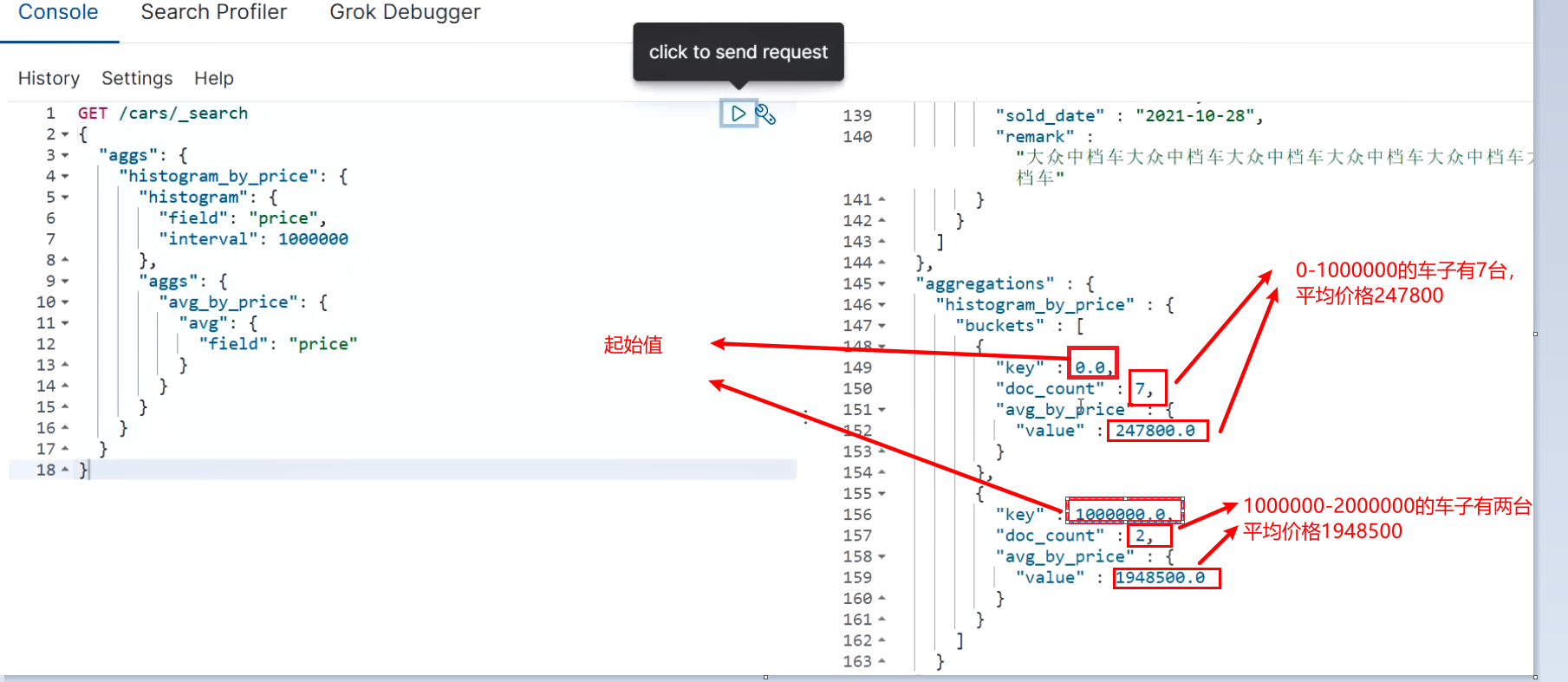
5.6 histogram interval statistics
histogram is similar to terms. It is also used for bucket grouping. It realizes data interval grouping according to a field.
For example, take 1 million as a range to count the sales volume and average price of vehicles in different ranges. When using histogram aggregation, the field specifies the price field price. The interval range is 1 million - interval: 1000000. At this time, ES will divide the price range into: [0, 1000000], [1000000, 2000000], [2000000, 3000000), etc., and so on. While dividing the range, histogram will count the data quantity similar to terms, and the aggregated data in the group can be aggregated and analyzed again through nested aggs.
GET /cars/_search
{
"aggs": {
"histogram_by_price": {
"histogram": {
"field": "price",
# The representative interval is 1000000, i.e. 0-100000010000001000000-20000002000000-3000000
"interval": 1000000
},
"aggs": {
"avg_by_price": {
"avg": {
"field": "price"
}
}
}
}
}
}
5.7 date_histogram interval grouping
date_histogram can perform interval aggregation grouping for date type field s, such as monthly sales, annual sales, etc.
For example, take the month as the unit to count the sales quantity and total sales amount of cars in different months. Date can be used at this time_ Histogram implements aggregation grouping, where field specifies the field used for aggregation grouping, interval (before es7) specifies the interval range (optional values are: year, quarter, month, week, day, hour, minute and second), and format specifies the date format, min_doc_count specifies the minimum number of documents for each interval (if not specified, the default is 0. When there is no document within the interval, the bucket group will also be displayed), extended_bounds specifies the start time and end time (if not specified, the range of the minimum value and the range of the maximum value in the field are the start time and end time by default).
ES7.x Previous syntax
GET /cars/_search
{
"aggs": {
"histogram_by_date" : {
"date_histogram": {
"field": "sold_date",
"interval": "month",
"format": "yyyy-MM-dd",
"min_doc_count": 1,
"extended_bounds": {
"min": "2021-01-01",
"max": "2022-12-31"
}
},
"aggs": {
"sum_by_price": {
"sum": {
"field": "price"
}
}
}
}
}
}
Appears after execution
#! Deprecation: [interval] on [date_histogram] is deprecated, use [fixed_interval] or [calendar_interval] in the future.

7.X after  interval Replace keyword with calendar_interval
GET /cars/_search
{
"aggs": {
"histogram_by_date" : {
"date_histogram": {
"field": "sold_date",
"calendar_interval": "month",
"format": "yyyy-MM-dd",
"min_doc_count": 1,
"extended_bounds": {
"min": "2021-01-01",
"max": "2022-12-31"
}
},
"aggs": {
"sum_by_price": {
"sum": {
"field": "price"
}
}
}
}
}
}
5.8 _global bucket
When aggregating statistics, it is sometimes necessary to compare some data with the overall data.
For example, make statistics on the average price of a brand of vehicles and the average price of all vehicles. Global is used to define a global bucket. This bucket ignores the query condition and retrieves all document s for corresponding aggregation statistics.
GET /cars/_search
{
"size" : 0,
"query": {
"match": {
"brand": "public"
}
},
"aggs": {
"volkswagen_of_avg_price": {
"avg": {
"field": "price"
}
},
"all_avg_price" : {
"global": {},
"aggs": {
"all_of_price": {
"avg": {
"field": "price"
}
}
}
}
}
}
5.9 aggs+order
Sort aggregate statistics.
For example, make statistics on the car sales and total sales of each brand, and arrange them in descending order of total sales.
GET /cars/_search
{
"aggs": {
"group_of_brand": {
"terms": {
"field": "brand",
"order": {
"sum_of_price": "desc"
}
},
"aggs": {
"sum_of_price": {
"sum": {
"field": "price"
}
}
}
}
}
}
If there are multiple aggs, you can also sort according to the innermost aggregation data when performing drill down aggregation.
For example, count the total sales of vehicles of each color in each brand and arrange them in descending order according to the total sales. This is just like grouping sorting in SQL. You can only sort the data within a group, not across groups.
GET /cars/_search
{
"aggs": {
"group_by_brand": {
"terms": {
"field": "brand"
},
"aggs": {
"group_by_color": {
"terms": {
"field": "color",
"order": {
"sum_of_price": "desc"
}
},
"aggs": {
"sum_of_price": {
"sum": {
"field": "price"
}
}
}
}
}
}
}
}
5.10 search+aggs
Aggregation is similar to the group by clause in SQL, and search is similar to the where clause in SQL. In ES, search and aggregations can be integrated to perform relatively more complex search statistics.
For example, make statistics on the sales volume and sales volume of a brand of vehicles in each quarter.
GET /cars/_search
{
"query": {
"match": {
"brand": "public"
}
},
"aggs": {
"histogram_by_date": {
"date_histogram": {
"field": "sold_date",
"calendar_interval": "quarter",
"min_doc_count": 1
},
"aggs": {
"sum_by_price": {
"sum": {
"field": "price"
}
}
}
}
}
}
5.11 filter+aggs
In ES, filter can also be combined with aggs to realize relatively complex filtering aggregation analysis.
For example, calculate the average price of vehicles between 100000 and 500000.
GET /cars/_search
{
"query": {
"constant_score": {
"filter": {
"range": {
"price": {
"gte": 100000,
"lte": 500000
}
}
}
}
},
"aggs": {
"avg_by_price": {
"avg": {
"field": "price"
}
}
}
}
5.12 using filter in aggregation
Filter can also be used in aggs syntax. The scope of filter determines its filtering scope.
For example, count the total sales of a brand of cars in the last year. Put the filter inside aggs, which means that the filter only performs filter filtering on the results obtained from query search. If the filter is placed outside the aggs, the filter will filter all the data.
- 12M/M means 12 months.
- 1y/y means 1 year.
- d stands for days
GET /cars/_search
{
"query": {
"match": {
"brand": "public"
}
},
"aggs": {
"count_last_year": {
"filter": {
"range": {
"sold_date": {
"gte": "now-12M"
}
}
},
"aggs": {
"sum_of_price_last_year": {
"sum": {
"field": "price"
}
}
}
}
}
}