Neural network and back propagation algorithm
4.1 cost function
in the previous section, we learned the basic structure of neural network and forward propagation algorithm. In the supporting operation, the weights of neural network have been given, but how can we train the appropriate weights ourselves? Therefore, we need to understand the cost function and back propagation algorithm.
we need to know some labeling methods. Suppose the neural network training samples have
m
m
m, each containing a set of inputs
x
x
x and a set of output signals
y
y
y,
L
L
L represents the number of neural network layers,
S
I
S_I
SI ^ represents the number of neurons in each layer,
S
L
S_L
SL ﹤ indicates the number of processing units in the last layer.
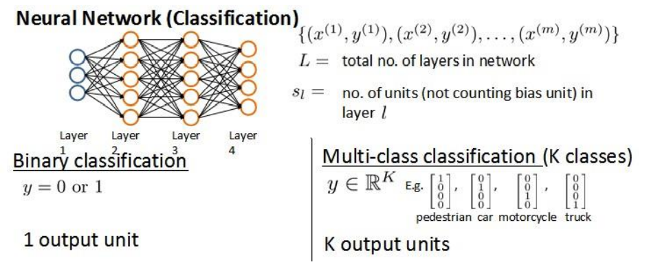
the classification of neural networks can be divided into two categories: Class II Classification and multi class classification. Class II Classification:
S
L
=
2
,
y
=
0
o
r
1
S_L=2,y=0 or 1
SL=2,y=0or1; Multi category classification:
S
L
=
k
,
y
i
=
1
S_L=k,y_i=1
SL = k,yi = 1 indicates the score to the second
i
i
Class i. (
k
>
2
k>2
k>2)
we review that the cost function in logistic regression is
J
(
θ
)
=
−
1
m
[
∑
i
=
1
n
y
(
i
)
l
o
g
h
θ
(
x
(
i
)
)
+
(
1
−
y
(
i
)
)
l
o
g
(
1
−
h
θ
(
x
(
i
)
)
)
]
+
λ
2
m
∑
j
=
1
n
θ
j
2
J(\theta)=-\frac{1}{m}[\sum_{i=1}^ny^{(i)}logh_\theta(x^{(i)})+(1-y^{(i)})log(1-h_\theta(x^{(i)}))]+\frac{\lambda}{2m}\sum_{j=1}^n\theta_j^2
J(θ)=−m1[i=1∑ny(i)loghθ(x(i))+(1−y(i))log(1−hθ(x(i)))]+2mλj=1∑nθj2
but because there are multiple outputs in the neural network, the cost function is more complex
h
Θ
(
x
)
∈
R
K
(
h
Θ
(
x
)
)
i
=
i
t
h
o
u
t
p
u
t
J
(
Θ
)
=
−
1
m
[
∑
i
=
1
m
∑
k
=
1
K
y
k
(
i
)
l
o
g
(
h
Θ
(
x
(
i
)
)
)
k
+
(
1
−
y
k
(
i
)
)
l
o
g
(
1
−
(
h
Θ
(
x
(
i
)
)
)
k
)
]
+
λ
2
m
∑
l
=
1
L
−
1
∑
i
=
1
s
l
∑
j
=
1
s
l
+
1
(
Θ
j
i
(
l
)
)
2
h_\Theta(x)\in \mathbb{R}^K\qquad (h_\Theta(x))_i=i^{th} output\\ J(\Theta)=-\frac{1}{m}[\sum_{i=1}^m\sum_{k=1}^Ky_k^{(i)}log(h_\Theta(x^{(i)}))_k+(1-y_k^{(i)})log(1-(h_\Theta(x^{(i)}))_k)]+\frac{\lambda}{2m}\sum_{l=1}^{L-1}\sum_{i=1}^{s_l}\sum_{j=1}^{s_{l+1}}(\Theta_{ji}^{(l)})^2
hΘ(x)∈RK(hΘ(x))i=ithoutputJ(Θ)=−m1[i=1∑mk=1∑Kyk(i)log(hΘ(x(i)))k+(1−yk(i))log(1−(hΘ(x(i)))k)]+2mλl=1∑L−1i=1∑slj=1∑sl+1(Θji(l))2
although the cost function is complex, the idea behind it is the same: we hope to know how far the prediction result of the algorithm is from the real situation by observing the cost function. Unlike logistic regression, neural networks have
K
K
For K predictions, we select the one with the highest possibility through circulation and compare it with
y
y
Compare the actual value in y. Similarly, we do not regularize the bias term, so
i
i
i start with 1.
4.2 back propagation algorithm
4.2.1 algorithm overview
in the forward propagation algorithm, we calculate layer by layer from the input layer
h
Θ
(
x
)
h_\Theta(x)
h Θ (x). Now let's calculate the partial derivative of the cost function
∂
∂
Θ
i
j
(
l
)
J
(
Θ
)
\frac{\partial}{\partial \Theta_{ij}^{(l)}}J(\Theta)
∂ Θ ij(l)∂J( Θ), We need to use the back-propagation algorithm, that is, first calculate the error of the last layer, and then calculate the error of each layer in reverse layer by layer until the penultimate layer. In my personal understanding, it is essentially the natural result of the chain derivation rule.
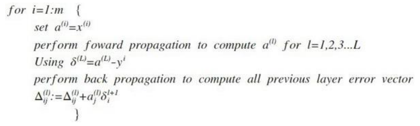
the example in the course is that there is only one training sample in the training set
(
x
(
1
)
,
y
(
1
)
)
(x^{(1)},y^{(1)})
(x(1),y(1)), the neural network structure is shown in the figure:
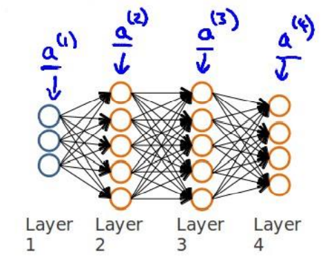
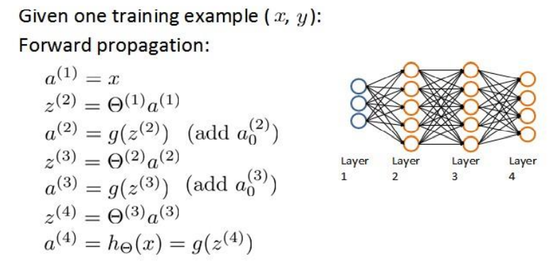
revisit the forward propagation algorithm:
we calculate the error from the last layer, which refers to the prediction of the activation unit(
a
k
(
4
)
a_k^{(4)}
ak(4)) and actual value(
y
k
y_k
Error between yk)
(
k
=
1
:
k
k=1:k
k=1:k), we use
δ
\delta
δ Represents the error, which we can understand temporarily here
δ
(
l
)
=
∂
∂
z
(
l
)
J
(
Θ
)
\delta^{(l)}=\frac{\partial}{\partial z^{(l)}}J(\Theta)
δ (l)=∂z(l)∂J( Θ), be
δ
(
4
)
=
a
(
4
)
−
y
\delta^{(4)}=a^{(4)}-y
δ (4)=a(4) − y, so we use this error value to calculate the error of the previous layer:
δ
(
3
)
=
∂
∂
z
(
3
)
J
(
Θ
)
=
∂
∂
z
(
4
)
J
(
Θ
)
⋅
∂
z
(
4
)
∂
a
(
3
)
⋅
∂
a
(
3
)
∂
z
(
3
)
=
(
Θ
(
3
)
)
T
δ
(
4
)
.
∗
g
′
(
z
(
3
)
)
\delta^{(3)}=\frac{\partial}{\partial z^{(3)}}J(\Theta)=\frac{\partial}{\partial z^{(4)}}J(\Theta)\cdot\frac{\partial z^{(4)}}{\partial a^{(3)}}\cdot\frac{\partial a^{(3)}}{\partial z^{(3)}}=(\Theta^{(3)})^T\delta^{(4)}.*g'(z^{(3)})
δ (3)=∂z(3)∂J( Θ)= ∂z(4)∂J( Θ) ⋅∂a(3)∂z(4)⋅∂z(3)∂a(3)=( Θ (3))T δ (4). * g '(z(3)), where
.
∗
.*
. * is point multiplication, corresponding element multiplication. Here is the chain rule in the derivation of composite function. Among them, we should also understand a property of sigmoid function:
g
′
(
z
)
=
g
(
z
)
∗
(
1
−
g
(
z
)
)
g'(z)=g(z)*(1-g(z))
g′(z)=g(z)∗(1−g(z)).
we can also get the error of the second layer:
δ
(
2
)
=
∂
∂
z
(
2
)
J
(
Θ
)
=
∂
∂
z
(
3
)
J
(
Θ
)
⋅
∂
z
(
3
)
∂
a
(
2
)
⋅
∂
a
(
2
)
∂
z
(
2
)
=
(
Θ
(
2
)
)
T
δ
(
3
)
.
∗
g
′
(
z
(
2
)
)
\delta^{(2)}=\frac{\partial}{\partial z^{(2)}}J(\Theta)=\frac{\partial}{\partial z^{(3)}}J(\Theta)\cdot\frac{\partial z^{(3)}}{\partial a^{(2)}}\cdot\frac{\partial a^{(2)}}{\partial z^{(2)}}=(\Theta^{(2)})^T\delta^{(3)}.*g'(z^{(2)})
δ(2)=∂z(2)∂J(Θ)=∂z(3)∂J(Θ)⋅∂a(2)∂z(3)⋅∂z(2)∂a(2)=(Θ(2))Tδ(3).∗g′(z(2))
with the expression of all errors, we can calculate the partial derivative of the cost function, assuming
λ
=
0
\lambda=0
λ= 0, that is, when we do not do regularization:
∂
∂
Θ
i
j
(
l
)
J
(
Θ
)
=
∂
∂
z
i
(
l
+
1
)
J
(
Θ
)
⋅
∂
z
i
(
l
+
1
)
∂
Θ
i
j
(
l
)
=
a
j
(
l
)
δ
(
l
+
1
)
\frac{\partial}{\partial \Theta_{ij}^{(l)}}J(\Theta)=\frac{\partial}{\partial z_i^{(l+1)}}J(\Theta)\cdot\frac{\partial z_i^{(l+1)}}{\partial \Theta_{ij}^{(l)}}=a_j^{(l)}\delta^{(l+1)}
∂Θij(l)∂J(Θ)=∂zi(l+1)∂J(Θ)⋅∂Θij(l)∂zi(l+1)=aj(l)δ(l+1)
In the above formula, the superscript and subscript mean:
l
l
l represents the layer currently calculated;
j
j
j represents the subscript of the active unit in the current computing layer;
i
i
i represents the subscript of the error unit in the next layer.
when there are many training samples in the training set and regularization processing is required, we use
Δ
i
j
(
l
)
\Delta_{ij}^{(l)}
Δ ij(l) is the total error, which means the sum of the partial derivatives of each sample without regularization. We express the algorithm as:
we cycle each sample, use the forward propagation algorithm to calculate the activation unit of each layer, and then use the back propagation method to calculate the error sum of multiple training samples. We also need to consider regularization, and finally obtain the partial derivative of the cost function:
D
i
j
(
l
)
=
1
m
(
Δ
i
j
(
l
)
+
λ
Θ
i
j
(
l
)
)
i
f
j
≠
0
D
i
j
(
l
)
=
1
m
Δ
i
j
(
l
)
i
f
j
=
0
D_{ij}^{(l)}=\frac{1}{m}(\Delta_{ij}^{(l)}+\lambda\Theta_{ij}^{(l)})\qquad if\quad j\neq0\\ D_{ij}^{(l)}=\frac{1}{m}\Delta_{ij}^{(l)}\qquad if\quad j=0
Dij(l)=m1(Δij(l)+λΘij(l))ifj=0Dij(l)=m1Δij(l)ifj=0
4.2.2 detail understanding
4.3 summary
4.3.1 random initialization
any optimization algorithm requires some initial parameters. We initialized the parameters to 0 earlier. Such an initial method is not feasible for neural networks. If we set all initial parameters to 0, it will mean that all active units in our second layer will have the same value. Similarly, if all our initial parameters are the same non-zero number, the result is the same.
we usually have an initial parameter of
±
ε
±\varepsilon
± ε Random value of.
def random_init(size):
    return np.random.uniform(-0.12, 0.12, size)
4.3.2 gradient inspection
compared with the first two learning algorithms, neural network will be more complex, so we may make some imperceptible errors in code implementation, which means that although the cost is decreasing, the final result may not be the optimal solution.
in order to avoid such problems, we adopt a numerical test method called gradient. Its essence is difference approximate differential. Select two very close points along the tangent direction in the cost function, and then calculate the average of the two points to estimate the gradient. For a particular
θ
\theta
θ, We calculated that
θ
−
ε
\theta-\varepsilon
θ − ε Chuhe
θ
+
ε
\theta+\varepsilon
θ+ε Generation value of(
ε
\varepsilon
ε Is a very small value, usually 0.001), and then the average of the two costs is used to estimate
θ
\theta
θ The value of the agency.
f
i
(
θ
)
≈
J
(
θ
(
i
+
)
)
+
J
(
θ
(
i
−
)
)
2
ε
f_i(\theta)≈\frac{J(\theta^{(i+)})+J(\theta^{(i-)})}{2\varepsilon}
fi(θ)≈2εJ(θ(i+))+J(θ(i−))
if the difference between the two is within a reasonable range, then the implementation of our algorithm is correct.
4.3.3 summary
if the number of hidden layers is greater than 1, ensure that the number of units in each hidden layer is the same. Generally, the more units in the hidden layer, the better. What we really need to decide is the number of hidden layers and the number of units in each middle layer.
- Random initialization of parameters
- Using forward propagation algorithm to calculate all h θ ( x ) h_\theta(x) hθ(x)
- Write calculation cost function J J J's code
- All partial derivatives are calculated by back propagation algorithm
- An optimization algorithm is used to minimize the cost function
4.4 Python implementation of supporting operations
4.4.1 review of the previous section
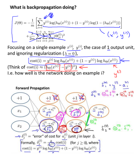
in this section, we also use handwritten data sets to implement BPNN
previously, we imported the library, visualized and read, and the weight has been given to propagate forward. The code is as follows, and the specific steps are shown in the previous section.
import matplotlib.pyplot as plt
import numpy as np
import scipy.io as sio
import matplotlib
import scipy.optimize as opt
from sklearn.metrics import classification_report#This package is the evaluation report


def load_data(path, transpose=True):
    data = sio.loadmat(path)
    y = data.get('y')  # (5000,1)
    y = y.reshape(y.shape[0])  # make it back to column vector

    X = data.get('X')  # (5000,400)

    if transpose:
        # for this dataset, you need a transpose to get the orientation right
        X = np.array([im.reshape((20, 20)).T for im in X])

        # and I flat the image again to preserve the vector presentation
        X = np.array([im.reshape(400) for im in X])

    return X, y

def expand_y(y):
    res = []
    for i in y:
        y_array = np.zeros(10)
        y_array[i-1] = 1
        res.append(y_array)
    return np.array(res)

def plot_100_image(X):
    """ sample 100 image and show them
    assume the image is square

    X : (5000, 400)
    """
    size = int(np.sqrt(X.shape[1]))

    # sample 100 image, reshape, reorg it
    sample_idx = np.random.choice(np.arange(X.shape[0]), 100)  # 100*400
    sample_images = X[sample_idx, :]

    fig, ax_array = plt.subplots(nrows=10, ncols=10, sharey=True, sharex=True, figsize=(8, 8))

    for r in range(10):
        for c in range(10):
            ax_array[r, c].matshow(sample_images[10 * r + c].reshape((size, size)),
                                   cmap=matplotlib.cm.binary)
            plt.xticks(np.array([]))
            plt.yticks(np.array([]))

X, _ = load_data('exdata1.mat', transpose=True)
plot_100_image(X)
plt.show()

X_raw, y_raw = load_data('ex4data1.mat', transpose=False)

X = np.insert(X_raw, 0, np.ones)
y = expand_y(y_raw)


def deserialize(seq):  # Disassembly parameters
    return seq[:25*401].reshape(25, 401), seq[25*401: ].reshape(10, 26)


def sigmoid(z):
    return 1 / (1 + np.exp(z))


def feed_forward(theta, X):  # Forward propagation
    t1, t2 = deserialize(theta)
    m = X.shape[0]
    a1 = X
    z2 = a1 @ t1.T
    a2 = np.insert(sigmoid(z2), 0, np.ones(m), axis=1)
    z3 = a2 @ t2.T
    h = sigmoid(z3)

    return a1, z2, a2, z3, h
4.4.2 cost function
J ( Θ ) = − 1 m [ ∑ i = 1 m ∑ k = 1 K y k ( i ) l o g ( h Θ ( x ( i ) ) ) k + ( 1 − y k ( i ) ) l o g ( 1 − ( h Θ ( x ( i ) ) ) k ) ] + λ 2 m ∑ l = 1 L − 1 ∑ i = 1 s l ∑ j = 1 s l + 1 ( Θ j i ( l ) ) 2 J(\Theta)=-\frac{1}{m}[\sum_{i=1}^m\sum_{k=1}^Ky_k^{(i)}log(h_\Theta(x^{(i)}))_k+(1-y_k^{(i)})log(1-(h_\Theta(x^{(i)}))_k)]+\frac{\lambda}{2m}\sum_{l=1}^{L-1}\sum_{i=1}^{s_l}\sum_{j=1}^{s_{l+1}}(\Theta_{ji}^{(l)})^2 J(Θ)=−m1[i=1∑mk=1∑Kyk(i)log(hΘ(x(i)))k+(1−yk(i))log(1−(hΘ(x(i)))k)]+2mλl=1∑L−1i=1∑slj=1∑sl+1(Θji(l))2
def regularized_cost(theta, X, y):  # Regularization cost function
    m = X.shape[0]
    t1, t2 = deserialize(theta)
    _, _, _, _, h = feed_forward(theta, X)
    pair_computation = -np.multiply(y, np.log(h)) - np.multiply((1-y), np.log(1-h))
    cost = pair_computation.sum() / m
    reg_t1 = (1 / (2*m)) * np.power(t1[:, 1:], 2).sum()
    reg_t2 = (1 / (2*m)) * np.power(t2[:, 1:], 2).sum()
    return cost + reg_t1 + reg_t2
4.4.3 back propagation algorithm
def serialize(a, b):  # Flattening parameters
    return np.concatenate((np.ravel(a), np.ravel(b)))

def sigmoid_gradient(z):
    return np.multiply(sigmoid(z), 1 - sigmoid(z))


def gradient(theta, X, y):
    t1, t2 = deserialize(theta)
    m = X.shape[0]

    delta1 = np.zeros(t1.shape)
    delta2 = np.zeros(t2.shape)

    a1, z2, a2, z3, h = feed_forward(theta, X)

    for i in range(m):
        a1i = a1[i, :]
        z2i = z2[i, :]
        z2i = np.insert(z2i, 0, np.ones(1), axis=0)
        a2i = a2[i, :]

        hi = h[i, :]
        yi = y[i, :]

        d3i = hi - yi
        d2i = np.multiply(t2.T @ d3i, sigmoid_gradient(z2i))

        delta2 += (1/m) * np.matrix(d3i).T @ np.matrix(a2i)  # Convert to matrix, (1,10) T@(1,26)->(10,26)
        delta1 += (1/m) * np.matrix(d2i[1:]).T @ np.matrix(a1i)  # (1,25).T@(1,401)->(25,401)

    t1[:, 0] = 0
    t2[:, 0] = 0
    reg_term1 = (1 / m) * t1
    reg_term2 = (1 / m) * t2
    delta2 += reg_term2
    delta1 += reg_term1
    return serialize(delta1, delta2)
4.4.4 gradient test
we use two norms to measure numerical and analytical gradients.
∥
n
u
m
e
r
i
c
a
l
_
g
r
a
d
−
a
n
a
l
y
t
i
c
_
g
r
a
d
∥
2
∥
n
u
m
e
r
i
c
a
l
_
g
r
a
d
∥
2
+
∥
a
n
a
l
y
t
i
c
_
g
r
a
d
∥
2
\frac{\Vert numerical\_grad - analytic\_grad\Vert_2}{\Vert numerical\_grad\Vert_2+\Vert analytic\_grad\Vert_2}
∥numerical_grad∥2+∥analytic_grad∥2∥numerical_grad−analytic_grad∥2
def expand_array(arr):
    """
    input [1,2,3]
    out
    [[1,2,3],
    [1,2,3],
    [1,2,3]]
    """
    return np.array(np.matrix(np.ones(arr.shape[0])).T @ np.matrix(arr))


def gradient_checking(theta, X, y, epsilon):
    def numeric_grad(plus, minus):
        return (regularized_cost(plus, X, y)-regularized_cost(minus, X, y)) / (2 * epsilon)

    theta_matrix = expand_array(theta)
    epsilon_matrix = np.identity(len(theta)) * epsilon

    plus_matrix = theta_matrix + epsilon_matrix
    minus_matrix = theta_matrix - epsilon_matrix

    numeric_grad = np.array([numeric_grad(plus_matrix[i], minus_matrix[i]) for i in range(len(theta))])
    analytic_grad = regularized_gradient(theta, X, y)

    diff = np.linalg.norm(numeric_grad - analytic_grad) / (np.linalg.norm(numeric_grad) + np.linalg.norm(analytic_grad))
    print("If your backpropagation implementation is correct,\n"
          "the relative difference will be smaller than 10e-7(assume epsilon=10e-7).\n"
          "Relative Difference:{}\n".format(diff))


def random_init(size):
    return np.random.uniform(-0.12, 0.12, size)


init_theta = random_init(10285)
gradient_checking(init_theta, X, y, epsilon=10e-7)
If your backpropagation implementation is correct,
the relative difference will be smaller than 10e-7(assume epsilon=10e-7).
Relative Difference:1.0262913293779404e-08
it should be noted that when the algorithm passes the gradient test, it must turn off the gradient test step before training the network, otherwise the training time is very long.
4.4.5 model training
def nn_training(X, y):
init_theta = random_init(10285)
res = opt.minimize(fun=regularized_cost,
x0=init_theta,
args=(X, y, 1),
method='TNC',
jac=regularized_gradient,
options={'maxiter': 400})
return res
res = nn_training(X, y)
_, y_answer = load_data('ex4data1.mat')
final_theta = res.x
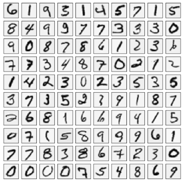
def show_accuracy(theta, X, y):
_, _, _, _, h = feed_forward(theta, X)
y_pred = np.argmax(h, axis=1) + 1
print(classification_report(y, y_pred))
show_accuracy(final_theta, X, y_answer)
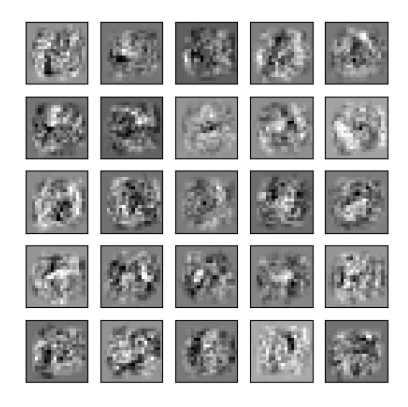
4.4.6 show hidden layers
def plot_hidden_layer(theta):
    final_theta1, _ = deserialize(theta)
    hidden_layer = final_theta1[:, 1:]

    fig, ax_array = plt.subplots(nrows=5, ncols=5, sharex=True, sharey=True, figsize=(5, 5))
    for r in range(5):
        for c in range(5):
            ax_array[r, c].matshow(hidden_layer[5*r + c].reshape(20, 20),
                                   cmap=matplotlib.cm.binary)
            plt.xticks([])
            plt.yticks([])


plot_hidden_layer(final_theta)
plt.show()