Refer to the official website: Scipy.

Fixed point problem

The problem closely related to finding the zero point of a function is to find the fixed point of a function. The fixed point of a function refers to the point returned when the function is evaluated: g ( x ) = x g(x)=x g(x)=x. Obviously, this is f ( x ) = g ( x ) − x f(x)=g(x)-x The zero point problem of f(x)=g(x) − X. fixed_point provides a simple iterative method, which uses Aitkens sequence acceleration to estimate g ( x ) g(x) The fixed point of g(x).

from scipy import optimize
import numpy as np
def func(x, c1, c2):
   return np.sqrt(c1/(x+c2))
c1 = np.array([10,12.])
c2 = np.array([3, 5.])
ans = optimize.fixed_point(func, [1.2, 1.3], args=(c1,c2))
print(ans)

The result is:

[1.4920333  1.37228132]

Root finding of univariate equation

For example:

import numpy as np
from scipy.optimize import root
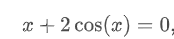
def func(x):
    return x + 2 * np.cos(x)
sol = root(func, 0.3)
print(sol.x)

The results are:

[-1.02986653]

Root finding of multivariable equation (method = 'lm')

For example:

import numpy as np
from scipy.optimize import root
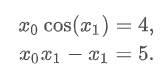
def func2(x):
    f = [x[0] * np.cos(x[1]) - 4,
         x[1]*x[0] - x[1] - 5]
    df = np.array([[np.cos(x[1]), -x[0] * np.sin(x[1])],
                   [x[1], x[0] - 1]])
    return f, df
sol = root(func2, [1, 1], jac=True, method='lm')
print(sol.x)

The results are:

[6.50409711 0.90841421]

Large scale root problem

hybr and lm cannot solve large-scale problems because they have to calculate n × N Jacobian matrix, with the increase of variables, the amount of calculation will be greater and greater.
For example, consider the following problems: we need to solve the following differential equations:

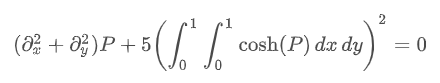
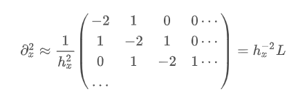
The limiting conditions are: the upper edge meets P ( x , 1 ) = 1 P(x,1)=1 P(x,1)=1, satisfied on the boundary P = 0 P=0 P=0. This can be achieved by approximating the continuous function p with the values on the grid (personal understanding is the finite difference method for fluid) P n , m ≈ P ( n h , m h ) P_{n,m}≈P(nh,mh) Pn,m​≈P(nh,mh). Then the derivative and integral can be approximated; For example:

In this way, large solvers can be used to solve: such as krylov, broyden2 and anderson. These methods use the so-called inexact Newton method, which does not accurately calculate the Jacobian matrix, but forms an approximate value.

import numpy as np
from scipy.optimize import root
from numpy import cosh, zeros_like, mgrid, zeros

# parameters
nx, ny = 75, 75
hx, hy = 1./(nx-1), 1./(ny-1)

P_left, P_right = 0, 0
P_top, P_bottom = 1, 0

def residual(P):
   d2x = zeros_like(P)
   d2y = zeros_like(P)

   d2x[1:-1] = (P[2:]   - 2*P[1:-1] + P[:-2]) / hx/hx
   d2x[0]    = (P[1]    - 2*P[0]    + P_left)/hx/hx
   d2x[-1]   = (P_right - 2*P[-1]   + P[-2])/hx/hx

   d2y[:,1:-1] = (P[:,2:] - 2*P[:,1:-1] + P[:,:-2])/hy/hy
   d2y[:,0]    = (P[:,1]  - 2*P[:,0]    + P_bottom)/hy/hy
   d2y[:,-1]   = (P_top   - 2*P[:,-1]   + P[:,-2])/hy/hy

   return d2x + d2y + 5*cosh(P).mean()**2

# solve
guess = zeros((nx, ny), float)
sol = root(residual, guess, method='krylov', options={'disp': True})
#sol = root(residual, guess, method='broyden2', options={'disp': True, 'max_rank': 50})
#sol = root(residual, guess, method='anderson', options={'disp': True, 'M': 10})
print('Residual: %g' % abs(residual(sol.x)).max())

# visualize
import matplotlib.pyplot as plt
x, y = mgrid[0:1:(nx*1j), 0:1:(ny*1j)]
plt.pcolormesh(x, y, sol.x, shading='gouraud')
plt.colorbar()
plt.show()

The result is:

0:  |F(x)| = 40.1231; step 1
1:  |F(x)| = 16.821; step 1
2:  |F(x)| = 5.69025; step 1
3:  |F(x)| = 1.41135; step 1
4:  |F(x)| = 0.0386739; step 1
5:  |F(x)| = 0.00171956; step 1
6:  |F(x)| = 0.000132096; step 1
7:  |F(x)| = 6.2608e-06; step 1
8:  |F(x)| = 3.69188e-07; step 1
Residual: 3.69188e-07

Acceleration method

For krylov method, most of its time is used to calculate the inverse of Jacobian matrix. If you have an approximation of the inverse matrix M ≈ J − 1 M≈J^{-1} M ≈ J − 1, then you can use it to preprocess the linear inversion problem.
We're not going to solve it J s = y Js=y Js=y, but solve it M J s = M y MJs=My MJs=My. Because the matrix is "closer" to the identity matrix than before, the Krylov method should be easier to deal with this equation.
Matrix M can be passed to Krylov method as an option options['jac_options']['inner_M '].
For the problem in the previous section, we notice that the function to be solved consists of two parts: the first part is Laplace operator and the second is integral. In fact, we can easily calculate the Jacobian coefficient corresponding to the Laplacian part:


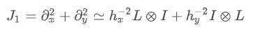
J 1 J_1 J1. You can use SciPy sparse. linalg. Splu (or approximate with scipy.sparse.linalg.splu). So we use M ≈ J 1 − 1 M≈J^{-1}_1 M ≈ J1 − 1 ≈ is pretreated to accelerate the calculation.

import numpy as np
from scipy.optimize import root
from scipy.sparse import spdiags, kron
from scipy.sparse.linalg import spilu, LinearOperator
from numpy import cosh, zeros_like, mgrid, zeros, eye

# parameters
nx, ny = 75, 75
hx, hy = 1./(nx-1), 1./(ny-1)

P_left, P_right = 0, 0
P_top, P_bottom = 1, 0

def get_preconditioner():
    """Compute the preconditioner M"""
    diags_x = zeros((3, nx))
    diags_x[0,:] = 1/hx/hx
    diags_x[1,:] = -2/hx/hx
    diags_x[2,:] = 1/hx/hx
    Lx = spdiags(diags_x, [-1,0,1], nx, nx)

    diags_y = zeros((3, ny))
    diags_y[0,:] = 1/hy/hy
    diags_y[1,:] = -2/hy/hy
    diags_y[2,:] = 1/hy/hy
    Ly = spdiags(diags_y, [-1,0,1], ny, ny)

    J1 = kron(Lx, eye(ny)) + kron(eye(nx), Ly)

    # Now we have the matrix `J_1`. We need to find its inverse `M` --
    # however, since an approximate inverse is enough, we can use
    # the *incomplete LU* decomposition

    J1_ilu = spilu(J1)

    # This returns an object with a method .solve() that evaluates
    # the corresponding matrix-vector product. We need to wrap it into
    # a LinearOperator before it can be passed to the Krylov methods:

    M = LinearOperator(shape=(nx*ny, nx*ny), matvec=J1_ilu.solve)
    return M

def solve(preconditioning=True):
    """Compute the solution"""
    count = [0]

    def residual(P):
        count[0] += 1

        d2x = zeros_like(P)
        d2y = zeros_like(P)

        d2x[1:-1] = (P[2:]   - 2*P[1:-1] + P[:-2])/hx/hx
        d2x[0]    = (P[1]    - 2*P[0]    + P_left)/hx/hx
        d2x[-1]   = (P_right - 2*P[-1]   + P[-2])/hx/hx

        d2y[:,1:-1] = (P[:,2:] - 2*P[:,1:-1] + P[:,:-2])/hy/hy
        d2y[:,0]    = (P[:,1]  - 2*P[:,0]    + P_bottom)/hy/hy
        d2y[:,-1]   = (P_top   - 2*P[:,-1]   + P[:,-2])/hy/hy

        return d2x + d2y + 5*cosh(P).mean()**2

    # preconditioner
    if preconditioning:
        M = get_preconditioner()
    else:
        M = None

    # solve
    guess = zeros((nx, ny), float)

    sol = root(residual, guess, method='krylov',
               options={'disp': True,
                        'jac_options': {'inner_M': M}})
    print('Residual', abs(residual(sol.x)).max())
    print('Evaluations', count[0])

    return sol.x

def main():
    sol = solve(preconditioning=True)

    # visualize
    import matplotlib.pyplot as plt
    x, y = mgrid[0:1:(nx*1j), 0:1:(ny*1j)]
    plt.clf()
    plt.pcolor(x, y, sol)
    plt.clim(0, 1)
    plt.colorbar()
    plt.show()


if __name__ == "__main__":
    main()

Good preprocessing may be crucial, and it can even determine whether the problem can be solved in practice.