Tutorial of the previous day: Directly create a separate conda environment for CellPhoneDB , and: Output the expression matrix and cell phenotype information in Seurat object to CellPhoneDB for cell communication , show you how to do cell communication for pbmc3k single cell data set, and in: Understanding of single cell communication results of CellPhoneDB The previous txt file shows you the meaning of multiple cell communication codes:
conda activate cellphonedb
cellphonedb method statistical_analysis test_meta.txt test_counts.txt  \
--counts-data hgnc_symbol --threads 4

# You must ensure that there is the out folder output in the previous steps under the current path
cellphonedb plot dot_plot
cellphonedb plot heatmap_plot cellphonedb_meta.txt
# After that, in order to distinguish from the previous ones, I changed the out folder to the out by symbol folder
Change the out folder to the out by symbol folder, and its structure is as follows:
ls -lh out-by-symbol|cut -d" " -f 7-

  1.5K  2 12 09:43 count_network.txt
   64K  2 12 09:30 deconvoluted.txt
   11K  2 12 09:43 heatmap_count.pdf
   11K  2 12 09:43 heatmap_log_count.pdf
  113B  2 12 09:43 interaction_count.txt
  149K  2 12 09:30 means.txt
  803K  2 12 09:43 plot.pdf
  128K  2 12 09:30 pvalues.txt
   61K  2 12 09:30 significant_means.txt
If your understanding of these documents is not enough, continue to read: Understanding of single cell communication results of CellPhoneDB
Next, we will carry out highly customized visualization of these files!
What we see with our naked eyes:
 all_sum
Memory_CD4_T 101
B 105
CD14_Mono 157
NK 171
CD8_T 100
Naive_CD4_T 68
FCGR3A_Mono 241
DC 180
Platelet 60
It's also monocytes, CD14_Mono and FCGR3A_ The total communication quantity of mono is different. Let's look at their communication with two kinds of CD4 T cells (Memory_CD4_T and Naive_CD4_T).
The main reason is that there are too many cell subsets. If all of them are visualized, it is difficult to explain them clearly.
rm(list = ls())
getwd()
setwd('pbmc3k-CellPhoneDB/')

mypvals <- read.table("./out-by-symbol/pvalues.txt",header = T,sep = "\t",stringsAsFactors = F)
mymeans <- read.table("./out-by-symbol/means.txt",header = T,sep = "\t",stringsAsFactors = F)
# Let's focus on CD14_Mono and FCGR3A_Mono, and Memory_CD4_T and Naive_CD4_T's communication.

kp = grepl(pattern = "Mono", colnames(mypvals)) & grepl(pattern = "CD4_T", colnames(mypvals))
table(kp)
pos = (1:ncol(mypvals))[kp]
choose_pvalues <- mypvals[,c(c(1,5,6,8,9),pos  )]
choose_means <- mymeans[,c(c(1,5,6,8,9),pos)]

logi <- apply(choose_pvalues[,5:ncol(choose_pvalues)]<0.05, 1, sum)
# Only some interaction pairs with cell specificity are retained
choose_pvalues <- choose_pvalues[logi>=1,]

# Remove null values
logi1 <- choose_pvalues$gene_a != ""
logi2 <- choose_pvalues$gene_b != ""
logi <- logi1 & logi2
choose_pvalues <- choose_pvalues[logi,]

# Keep choose under the same conditions_ means
choose_means <- choose_means[choose_means$id_cp_interaction %in% choose_pvalues$id_cp_interaction,]
Two variables, choose, are obtained as follows_ Means and choose_pvalues, the five columns in front of them are the same, but there are only eight columns behind them, not 16 columns of 4X4, indicating that there are no statistically significant cell communication receptors and ligands between the two combinations of many single-cell subsets.
> head(choose_means,1)
   id_cp_interaction gene_a gene_b receptor_a receptor_b CD14_Mono.Memory_CD4_T CD14_Mono.Naive_CD4_T
40   CPI-SS0703338F5 LGALS9   CD44      False       True                  0.862                 0.803
   FCGR3A_Mono.Memory_CD4_T FCGR3A_Mono.Naive_CD4_T Memory_CD4_T.CD14_Mono Memory_CD4_T.FCGR3A_Mono
40                    0.949                    0.89                  0.552                     0.71
   Naive_CD4_T.CD14_Mono Naive_CD4_T.FCGR3A_Mono
40                 0.513                    0.67


> head(choose_pvalues,1)
   id_cp_interaction gene_a gene_b receptor_a receptor_b CD14_Mono.Memory_CD4_T CD14_Mono.Naive_CD4_T
40   CPI-SS0703338F5 LGALS9   CD44      False       True                      0                     0
   FCGR3A_Mono.Memory_CD4_T FCGR3A_Mono.Naive_CD4_T Memory_CD4_T.CD14_Mono Memory_CD4_T.FCGR3A_Mono
40                        0                       0                  0.888                        0
   Naive_CD4_T.CD14_Mono Naive_CD4_T.FCGR3A_Mono
40                     1                       1
It can be seen that there were 302 rows and more than 90 columns before, that is, 9 cell subsets, each communicating with 9 single cell subsets including yourself. The analysis results show that there are 81 pairwise combinations, but now there are only 8 single cell subsets, and only 19 receptor ligands, right:
> dim(mypvals)
[1] 302  92
> dim(mymeans)
[1] 302  92
> dim(choose_means)
[1] 19 13
> dim(choose_pvalues)
[1] 19 13
Next, we will simply visualize the results of the combination of these 19 receptor ligand pairs in 8 single-cell subsets. Although it is simple, the code is also a little long:
# choose_pvalues and choose_means data width to length
library(tidyverse)
meansdf <- choose_means %>% reshape2::melt()
meansdf <- data.frame(interacting_pair = paste0(meansdf$gene_a,"_",meansdf$gene_b),
                      CC = meansdf$variable,
                      means = meansdf$value)
pvalsdf <- choose_pvalues %>% reshape2::melt()
pvalsdf <- data.frame(interacting_pair = paste0(pvalsdf$gene_a,"_",pvalsdf$gene_b),
                      CC = pvalsdf$variable,
                      pvals = pvalsdf$value)

# Merge p value and mean file
pvalsdf$joinlab<- paste0(pvalsdf$interacting_pair,"_",pvalsdf$CC)
meansdf$joinlab<- paste0(meansdf$interacting_pair,"_",meansdf$CC)
pldf <- merge(pvalsdf,meansdf,by = "joinlab")

# dotplot visualization
summary((filter(pldf,means >0))$means)
head(pldf)
pcc =  pldf%>% filter(means >0) %>%
  ggplot(aes(CC.x,interacting_pair.x) )+
  geom_point(aes(color=means,size=-log10(pvals+0.0001)) ) +
  scale_size_continuous(range = c(1,3))+
  scale_color_gradient2(high="red",mid = "yellow",low ="darkblue",midpoint = 1  )+
  theme_bw()+
  # scale_color_manual(values = rainbow(100))+
  theme(axis.text.x = element_text(angle = -45,hjust = -0.1,vjust = 0.8))
pcc
As follows:
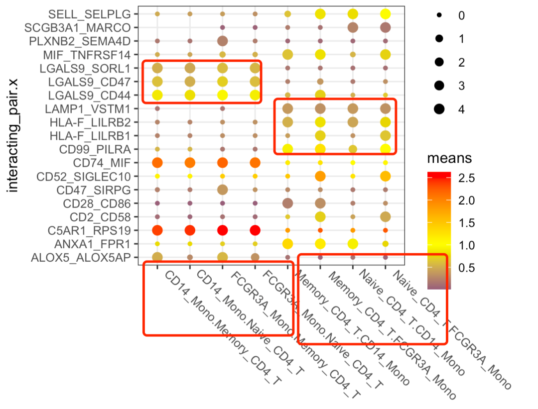
It can be seen that the receptor ligand pairs from mono to cd4 are basically completely different from those from cd4 to mono. The specific information of these 19 receptor ligand pairs is shown below
> unique(pldf$interacting_pair.x)
 [1] "ALOX5_ALOX5AP" "ANXA1_FPR1"    "C5AR1_RPS19"   "CD2_CD58"      "CD28_CD86"     "CD47_SIRPG"
 [7] "CD52_SIGLEC10" "CD74_MIF"      "CD99_PILRA"    "HLA-F_LILRB1"  "HLA-F_LILRB2"  "LAMP1_VSTM1"
[13] "LGALS9_CD44"   "LGALS9_CD47"   "LGALS9_SORL1"  "MIF_TNFRSF14"  "PLXNB2_SEMA4D" "SCGB3A1_MARCO"
[19] "SELL_SELPLG"
And, to the naked eye, it's CD74_MIF and c5ar1_ The RPS19 pairing is obvious. Let's look at their expression. The code is as follows:
library(SeuratData) #Load the seurat dataset
getOption('timeout')
options(timeout=10000)
#InstallData("sce")
data("pbmc3k")
sce <- pbmc3k.final
library(Seurat)
table(Idents(sce))
sce = sce[,Idents(sce) %in% c('Naive CD4 T', 'Memory CD4 T' ,  'CD14+ Mono','FCGR3A+ Mono')]
DimPlot(sce,label = T,repel = T)

cg = unique(unlist(str_split(unique(pldf[,2]),'_')) )

library(ggplot2)
th=  theme(axis.text.x = element_text(angle = -45,hjust = -0.1,vjust = 0.8))
pdopt <- DotPlot(sce, features = cg,
              assay='RNA'  )  + coord_flip() +th
library(patchwork)
pdopt + DimPlot(sce,label = T,repel = T)
pdopt + pcc
The results are as follows:
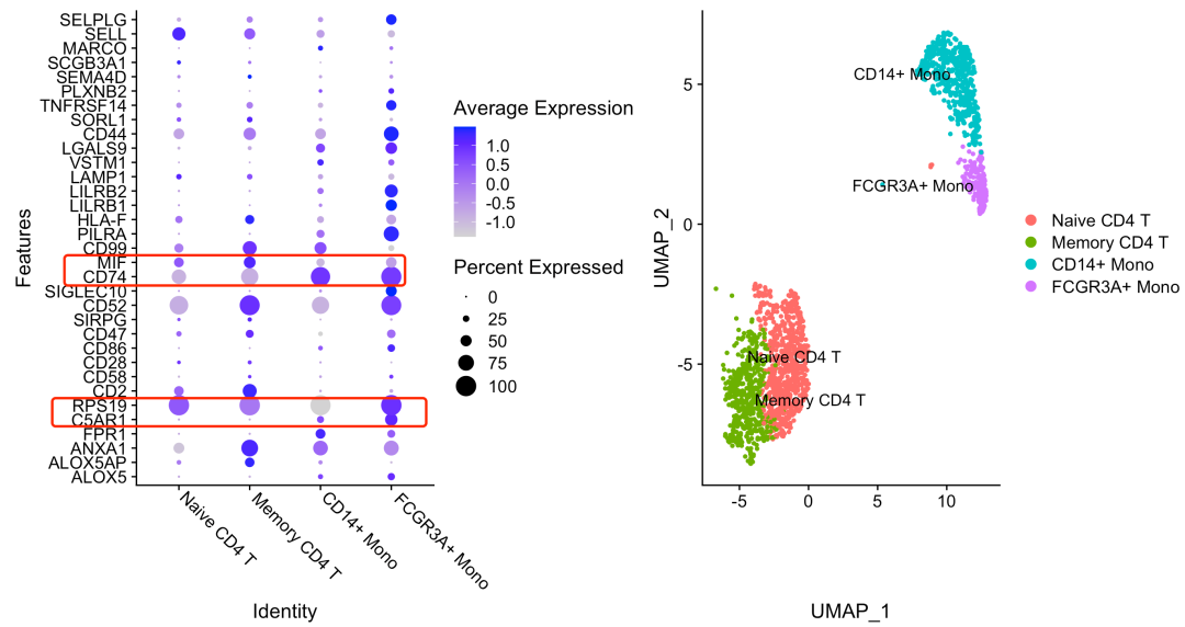
Isn't it very simple, CD74 in front_ MIF and C5AR1_ The pairing of RPS19 is obvious in the direction from mono to cd4, so CD74 and C5AR1 are highly expressed in mono, while MIF and RPS19 are highly expressed in cd4 T cells.
The so-called cell communication is the differential analysis from one gene unit to two genes
We can easily find the high expression genes of different single-cell subsets by differential analysis, but these genes are an independent list in each single-cell subset. The so-called single-cell communication is to find the pairwise combinations of specific genes of different single-cell subsets, and those with the biological background knowledge of receptor ligands.