0 research background
Write before:
1. This code is based on MATLAB2019a. Errors may be reported in the lower version or different versions, and the opening of mdl file or slx file may fail;
2. If the running time is too long, observe whether the number of iterations changes.
3. This blog is attached with the code and detailed introduction. If you reprint it, please indicate the source;
4. If this blog happens to be related to your research, you are welcome to consult qq1366196286;
Reference blog
[Simulink] PSO optimization algorithm for tuning PID controller parameters (I)
[Simulink] GA optimization algorithm for tuning PID controller parameters (III) -- first-order controlled object with time delay
continue to explain this blog: [Simulink] NSGA-2 optimization algorithm tuning PID controller parameters (IV) -- first-order controlled object with time delay
1. Brief introduction of multi-objective optimization algorithm
for the basic concept, please refer to the literature:
[1] Deb K, Pratap A, Agarwal S, et al. A fast and elitist multiobjective genetic algorithm: NSGA-II[J]. IEEE Transactions on Evolutionary Computation, 2002, 6(2):182-197.
[2] Zhang Q, Li H. MOEA/D: A Multiobjective Evolutionary Algorithm Based on Decomposition[J]. IEEE Transactions on Evolutionary Computation, 2007, 11(6):712-731.
1.1 brief introduction of nsga-2 algorithm
NSGA - Ⅱ is one of the most popular multi-objective genetic algorithms at present. It reduces the complexity of non inferior sorting genetic algorithm. It has the advantages of fast running speed and good convergence of solution set. It has become the benchmark of the performance of other multi-objective optimization algorithms.
NSGA - Ⅱ is improved on the basis of the first generation non dominated sorting genetic algorithm. Its improvement is mainly aimed at the three aspects mentioned above:
① A fast non dominated sorting algorithm is proposed. On the one hand, it reduces the computational complexity. On the other hand, it combines the parent population with the child population, so that the next generation population can be selected from double space, so as to retain all the best individuals;
② The elite strategy is introduced to ensure that some excellent population individuals will not be discarded in the process of evolution, so as to improve the accuracy of optimization results;
③ The use of crowding degree and crowding degree comparison operator not only overcomes the defect of manually specifying shared parameters in NSGA, but also takes it as the comparison standard between individuals in the population, so that the individuals in the quasi Pareto domain can be evenly extended to the whole Pareto domain, and the diversity of the population is guaranteed.
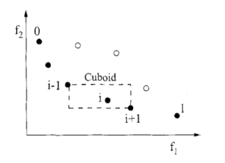
Figure 4-1 calculation of congestion degree and congestion distance
Algorithm purpose:
For the current m individuals, select N individuals (M > N).
NSGA-II key algorithm (steps):
1. First find the pareto solution for M individuals. Then we get the set of these pareto, such as F1, F2.
2. Put all individuals of F1 into N. if N is not full, continue to put F2 until Fk cannot be put into N (space) that has been put into F1, F2,..., F(k-1). Fk is solved at this time.
3. For individuals in FK, find the crowding distance Lk[i](crowding distance) of each individual in FK, sort it in descending order according to Lk[i] in FK, and put it into N until N is full.
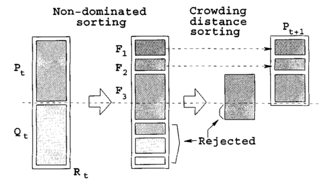
Figure 4-2 generation of parents and offspring of NSGA-II
Among them, NSGA-II key subroutine algorithm
1) Fast non dominated sorting algorithm
the key of multi-objective optimization problem is to find the Pareto optimal solution set. NSGA-II fast non dominated sorting is to obtain Fi by layering the population m according to the individual non inferior solution level, which is used to make the solution close to the Pareto optimal solution. This is a cyclic fitness grading process. First, find the non dominated solution set in the group, record it as F1, assign all its individuals to the non dominated order irank=1 (where irank is the non dominated order value of individual i), remove it from the whole group M, and then continue to find the non dominated solution set in the remaining group, record it as F2, and the individuals in F2 are given irank=2, It is known that the whole population is stratified, and the non dominated order value in Fi layer is the same.
2) Individual crowding distance
selective sorting is required in the same layer Fk, which is sorted according to the size of individual crowding distance. Individual crowding distance is the distance between individuals i+1 and i-1 adjacent to i on Fk. Its calculation steps are as follows:
① Initialize the individual distance of the same layer so that L[i]d=0 (represents the congestion distance of any individual I).
② The individuals in the same layer are arranged in ascending order according to the value of the m-th objective function.
③ Individuals on the edge of ranking should be given a choice advantage.
④ For the individuals in the middle of the ranking, calculate the crowding distance:
⑤ For different objective functions, repeat steps ② to ④ to obtain the crowding distance L[i]d of individual I. limited selection of individuals with large crowding distance can make the calculation results evenly distributed in the target space and maintain the diversity of the population.
3) Elite strategy selection algorithm
keep the excellent individuals in the parent generation directly into the offspring to prevent the loss of Pareto optimal solution. Select the index to optimize the population Ri synthesized by parent Ci and offspring Di to form a new parent Ci+1 First eliminate the scheme whose scheme test flag is infeasible in the parent generation, and then put the whole layer of population into Ci+1 from low to high according to the non dominated order value irank until Fk in a certain layer exceeds the limit of N. finally, fill Ci+1 according to the crowding distance until the population number is n.
among them, Figure 4-3 shows the Pareto front of the double objective function, in which the smaller the objective functions f1 and f2, the better. The solid line and the dotted line constitute the feasible region. The solid line represents the Pareto frontier, that is, the surface composed of the target vectors corresponding to all Pareto optimal solutions. A multi-objective optimization problem corresponds to a Pareto frontier. In addition, points a, B and C are located on the Pareto front. The solutions of these three points are Pareto optimal solutions, and there is no dominant or dominant relationship among them. D. The solutions of points E and F are feasible solutions and non Pareto optimal solutions. The solution of point a dominates the solution of point F, or the solution of point a is Pareto dominant compared with the solution of point F. Similarly, there is a dominant or dominant relationship between points B and C and points D, e and F.
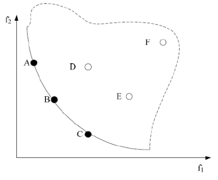
Figure 4-3 Pareto front of non dominated solution under double objective function
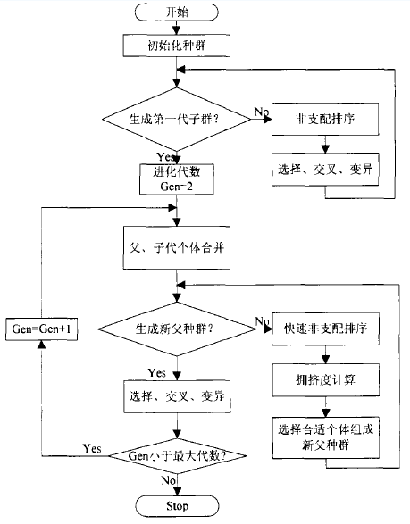
Figure 4-4 general steps of NSGA-II algorithm
Pseudo code of NSGA-2 algorithm
Pseudo code of sorting algorithm
def  fast_nondominated_sort( P ):
    F  =  [ ]
     for  p  in  P:
        Sp  =  [ ]
         np  =  0
          for  q  in  P:
              if  p  >  q:                 # If p dominates q, add q to the Sp list
                 Sp.append( q )
              else   if  p  <  q:         # If p is dominated by q, add np to 1
                 np  +=   1

         if  np  ==  0:
            p_rank  =   1          # If the individual's np is 0, the individual is Pareto level 1
      F1.append( p )
    F.append( F1 )
    i  =  0
     while  F[i]:
        Q  =  [ ]
         for  p  in  F[i]:
             for  q  in  Sp:         # Sort all individuals in the Sp set
                nq  -=   1
                 if  nq  ==  0:      # If the dominant number of the individual is 0, the individual is a non dominant individual
                    q_rank  =  i + 2      # The individual Pareto level is the current highest level plus 1. At this time, the initial value of i is 0, so add 2
                    Q.append( q )
        F.append( Q )
        i  +=   1
Pseudocode of individual crowding distance operator
def  crowding_distance_assignment( I )
        nLen  =  len( I )         # Number of individuals in I
     for  i  in  I:
                i.distance  =  0     # Initialize the crowding distance of all individuals
     for  objFun  in  M:         # M is the list of all objective functions
                I  =  sort( I, objFun )     # Sort in ascending order according to the objective function objFun
                I[0]  =  I[ len[I] - 1  ]  =  ∞     # Set the distance between the first and last individuals to infinity
                 for  i  in  xrange(  1 , len(I)  -   2  ):
                        I[i].distance  =  I[i].distance  +  ( objFun( I[i + 1 ] )  -  objFun( I[i - 1 ] ) ) / (Max(objFun())  -  Min(objFun()) )
1.3 case implementation of nsga-2 algorithm
this blog posts the Matlab implementation of NSGA - Ⅱ algorithm (the test function is ZDT1), the original link: Matlab implementation of NSGA - Ⅱ algorithm (the test function is ZDT1)
The first test function ZDT1
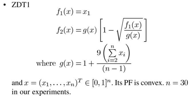
Figure 4-5 test function ZDT1
The code is as follows:
function f = evaluate_objective(x, M, V)
f = [];
f(1) = x(1);
g = 1;
sum = 0;
for i = 2:V
    sum = sum + x(i);
end
g = g + 9*sum / (V-1));
f(2) = g * (1 - sqrt(x(1) / g));
end
The NSGA2 code is implemented as follows:
function NSGAII()
clc;
format compact;
tic;
hold on

%---initialization/Parameter setting

    generations=100;                                %Number of iterations
    popnum=100;                                     %Population size(Must be even)
    poplength=30;                                   %Individual length
    minvalue=repmat(zeros(1,poplength),popnum,1);   %Individual minimum
    maxvalue=repmat(ones(1,poplength),popnum,1);    %Individual maximum
    population=rand(popnum,poplength).*(maxvalue-minvalue)+minvalue;    %Generate a new initial population

%---Start iterative evolution

    for gene=1:generations                      %Start iteration

%-------overlapping

        newpopulation=zeros(popnum,poplength);  %Offspring population
        for i=1:popnum/2                        %Cross generation offspring
            k=randperm(popnum);                 %Two parents were randomly selected from the population,Binary League method is not used
            beta=(-1).^round(rand(1,poplength)).*abs(randn(1,poplength))*1.481; %The normal distribution is used to cross produce two offspring
            newpopulation(i*2-1,:)=(population(k(1),:)+population(k(2),:))/2+beta.*(population(k(1),:)-population(k(2),:))./2;    %Produce the first generation
            newpopulation(i*2,:)=(population(k(1),:)+population(k(2),:))/2-beta.*(population(k(1),:)-population(k(2),:))./2;      %Produce the second generation
        end

%-------variation

        k=rand(size(newpopulation));    %Randomly select the loci to be mutated
        miu=rand(size(newpopulation));  %Polynomial variation
        temp=k<1/poplength & miu<0.5;   %Loci to be mutated
        newpopulation(temp)=newpopulation(temp)+(maxvalue(temp)-minvalue(temp)).*((2.*miu(temp)+(1-2.*miu(temp)).*(1-(newpopulation(temp)-minvalue(temp))./(maxvalue(temp)-minvalue(temp))).^21).^(1/21)-1);        %Variation I
        newpopulation(temp)=newpopulation(temp)+(maxvalue(temp)-minvalue(temp)).*(1-(2.*(1-miu(temp))+2.*(miu(temp)-0.5).*(1-(maxvalue(temp)-newpopulation(temp))./(maxvalue(temp)-minvalue(temp))).^21).^(1/21));  %Variation II

%-------Cross border processing/Population merging

        newpopulation(newpopulation>maxvalue)=maxvalue(newpopulation>maxvalue); %Offspring over upper bound processing
        newpopulation(newpopulation<minvalue)=minvalue(newpopulation<minvalue); %Offspring cross lower bound processing
        newpopulation=[population;newpopulation];                               %Combined parent-child population

%-------Calculate the objective function value

        functionvalue=zeros(size(newpopulation,1),2);           %Objective function values of the combined population,The problem here is ZDT1
        functionvalue(:,1)=newpopulation(:,1);                  %Calculate the value of the first dimensional objective function
        g=1+9*sum(newpopulation(:,2:poplength),2)./(poplength-1);
        functionvalue(:,2)=g.*(1-(newpopulation(:,1)./g).^0.5); %Calculate the value of the second objective function

%-------Non dominated sorting

        fnum=0;                                             %Currently assigned leading edge number
        cz=false(1,size(functionvalue,1));                  %Record whether the individual has been assigned a number
        frontvalue=zeros(size(cz));                         %Leading edge number of each individual
        [functionvalue_sorted,newsite]=sortrows(functionvalue);    %Sort the population according to the target value of the first dimension
        while ~all(cz)                                      %Start iteratively judging the frontiers of each individual,Adopt improved deductive sort
            fnum=fnum+1;
            d=cz;
            for i=1:size(functionvalue,1)
                if ~d(i)
                    for j=i+1:size(functionvalue,1)
                        if ~d(j)
                            k=1;
                            for m=2:size(functionvalue,2)
                                if functionvalue_sorted(i,m)>functionvalue_sorted(j,m)
                                    k=0;
                                    break
                                end
                            end
                            if k
                                d(j)=true;
                            end
                        end
                    end
                    frontvalue(newsite(i))=fnum;
                    cz(i)=true;
                end
            end
        end

%-------Calculate congestion distance/Select the next generation of individuals

        fnum=0;                                                                 %Current frontier
        while numel(frontvalue,frontvalue<=fnum+1)<=popnum                      %Judge how many individuals of the first face can be completely put into the next generation population
            fnum=fnum+1;
        end
        newnum=numel(frontvalue,frontvalue<=fnum);                              %front fnum Number of individuals per face
        population(1:newnum,:)=newpopulation(frontvalue<=fnum,:);               %Before fnum Individual faces are copied into the next generation
        popu=find(frontvalue==fnum+1);                                          %popu Record No fnum+1 Individual number on one face
        distancevalue=zeros(size(popu));                                        %popu Crowding distance of each individual
        fmax=max(functionvalue(popu,:),[],1);                                   %popu Maximum value per dimension
        fmin=min(functionvalue(popu,:),[],1);                                   %popu Minimum value per dimension
        for i=1:size(functionvalue,2)                                           %Sub target calculation on each target popu Crowding distance of each individual
            [~,newsite]=sortrows(functionvalue(popu,i));
            distancevalue(newsite(1))=inf;
            distancevalue(newsite(end))=inf;
            for j=2:length(popu)-1
                distancevalue(newsite(j))=distancevalue(newsite(j))+(functionvalue(popu(newsite(j+1)),i)-functionvalue(popu(newsite(j-1)),i))/(fmax(i)-fmin(i));
            end
        end
        popu=-sortrows(-[distancevalue;popu]')';                                %Ranked in descending order of crowding distance fnum+1 Individual on one face
        population(newnum+1:popnum,:)=newpopulation(popu(2,1:popnum-newnum),:);	%Will be the first fnum+1 Front with large crowding distance popnum-newnum Individuals are copied into the next generation
    end

%---Program output

    fprintf('Completed,time consuming%4s second\n',num2str(toc));          %The final time of the program
    output=sortrows(functionvalue(frontvalue==1,:));    %final result:Function value of non dominated solution in population
    plot(output(:,1),output(:,2),'*b');                 %Mapping
    axis([0,1,0,1]);xlabel('F_1');ylabel('F_2');title('ZDT1')
end
The running result is shown in the following figure:
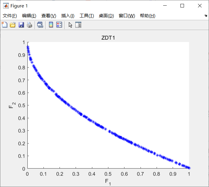
Figure 4-6 example implementation results of nsga-2 algorithm
Second test function
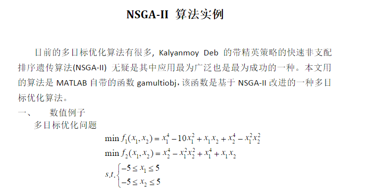
The code implementation of the test function is as follows:
function y=f(x)
y(1)=x(1)^4-10*x(1)^2+x(1)*x(2)+x(2)^4-x(1)^2*x(2)^2
y(2)=x(2)^4-x(1)^2*x(2)^2+x(1)^4+x(1)*x(2)
The code implementation of NSGA-2 MATLAB built-in function is as follows:
% At present, there are many multi-objective optimization algorithms,?Kalyanmoy?Deb Fast non dominated sorting genetic algorithm with elite strategy(NSGA-II)
%It is undoubtedly the most widely used and successful one. The algorithm used in this paper is MATLAB Self contained function gamultiobj,Based on this function NSGA-II An improved multi-objective optimization algorithm.

clc;
clear all;
fitnessfcn=@object_fun;  %Fitness function handle,objective function
nvars=2;                 %Number of variables x1 x2
lb=[-5,-5];              %lower limit
ub=[5,5];                %upper limit
A=[];
b=[];                    %Linear inequality constraint
Aeq=[];
beq=[];                  %linear equality constraint
options=gaoptimset('paretoFraction',0.3,'populationsize',500,'generations',200,...
    'stallGenLimit',200,'TolFun',1e-100,'PlotFcns',@gaplotpareto);
%Optimal individual coefficient paretoFaction Is 0.3;Population size populationsize Is 100,
%Maximum evolutionary algebra generations Stop algebra for 200 stallGenlimit 200,
%Fitness function deviation TolFun Set to 1 e-100 function gaplotpareto: draw Pareto front end
[x,fval]=gamultiobj(fitnessfcn,nvars,A,b,Aeq,beq,lb,ub,options)   %MATLAB Self contained function gamultiobj
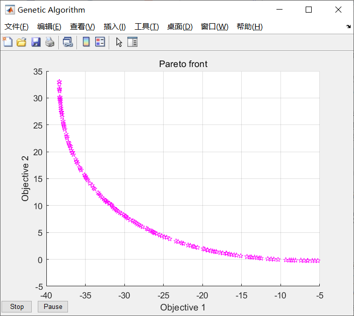
Figure 4-7 implementation result of nsga-2 matlab function
2 design of controlled object and fitness function
Introduction of controlled object
taking the transfer function of the second-order type I time-delay system as an example, the NSGA-2 algorithm is used to optimize the PID parameters, in which the system is set as the sampling time of 1 ms, the instruction is the unit step signal, and the simulation running time is 1.0 s. Among them, the performance optimization function is Best_J adopts the Integral of Time Multiplied by the Absolute Value of Error (ITAE). At the same time, in order to avoid overshoot caused by too large control quantity, in the performance optimization function best_ Add the square term of PID controller input to J. This is only the fitness function of one of the objectives. In addition, it is necessary to design the fitness function of other objectives, such as the design of fitness function in 2.2.
the transfer function of second-order type I delay system is as follows. It can be designed according to its own actual system m document

2.2 design of fitness function
(1) Objective fitness function 1
in order to obtain a satisfactory transition process, the absolute value of error time integration performance index is used as the fitness evaluation function Best_J. At the same time, in order to prevent the control input from being too large, in Best_J add the scoring item of control input, as shown in formula (1-2).

In equation (1-2), e(t) is the system output error, and u(t) is the input of PID controller, ρ 1, ρ 2 is the weight value.
in order to avoid overshoot, the penalty function is used to give priority to the overshoot, as shown in equation (1-3).

In formula (1-3) ρ 3>>max( ρ 1, ρ 2 and ρ 4) , and y(t) is the output of the controlled object, ey(t)=y(t)-y(t-1).
This is the design of the first objective fitness function.
(2) Objective fitness function 2
The rise time, adjustment time and delay time of the system are superimposed according to the principle of time minimization to construct the design of the second objective fitness function.
3PID parameter setting
3.1 PID parameter tuning of nsga-2 algorithm
%%%%%%%%%%%%%%%%%%%%%%%%%%%%%%%%%%%%%%%%%%%%%%%%%%%%%%
global rin yout timef
pop = 500; %Population number
gen = 100; %Number of iterations
M = 2;  %Target quantity
V = 3;   %dimension

MinX(1) = 0*ones(1); %Kp
MaxX(1) = 30*ones(1);

MinX(2) = 0*ones(1); %Kp
MaxX(2) = 1.0*ones(1);

MinX(3) = 0*ones(1); %Kp
MaxX(3) = 1.0*ones(1);

min_range = [MinX(1) MinX(2) MinX(3)]; %Lower bound
max_range = [MaxX(1) MaxX(2) MaxX(3)];   %upper bound

%% initialization
chromosome = initialize_variables(pop, M, V, min_range, max_range);
%Non dominated quick sequencing and congestion calculation are carried out for the initial population

chromosome = non_domination_sort_mod(chromosome, M, V);

%% Main program loop
for i = 1 : gen
pool = round(pop/2); %Mating pool size
tour = 2;            %Number of contestants in the bidding competition
%Selection of parents suitable for breeding in the competition
parent_chromosome = tournament_selection(chromosome, pool, tour);
mu = 20;
mum = 20;
offspring_chromosome = genetic_operator(parent_chromosome,M, V, mu, mum, min_range, max_range);
[main_pop,~] = size(chromosome);
[offspring_pop,~] = size(offspring_chromosome);
clear temp
intermediate_chromosome(1:main_pop,:) = chromosome;
intermediate_chromosome(main_pop + 1 : main_pop + offspring_pop,1 : M+V) = offspring_chromosome;
intermediate_chromosome = non_domination_sort_mod(intermediate_chromosome, M, V);
chromosome = replace_chromosome(intermediate_chromosome, M, V, pop);
    if ~mod(i,100)
    clc;
    fprintf('%d generations completed\n',i);
    end
end
figure(1);
if M == 2
plot(chromosome(:,V + 1),chromosome(:,V + 2),'*');
xlabel('f_1'); ylabel('f_2');
title('Pareto Optimal Front');
elseif M == 3
plot3(chromosome(:,V + 1),chromosome(:,V + 2),chromosome(:,V + 3),'*');
xlabel('f_1'); ylabel('f_2'); zlabel('f_3');
title('Pareto Optimal Surface');
end
figure(2);
plot(timef,rin,'r',timef,yout,'b');
xlabel('Time(s)');ylabel('rin,yout');


%% //*******Subroutine initialize_variables**********//
function f = initialize_variables(N, M, V, min_range, max_range)
min = min_range;
max = max_range;

K = M + V;

    for i = 1 : N

        for j = 1 : V

        f(i,j) = min(j) + (max(j) - min(j))*rand(1);
        end
        Kpidi=f(i,:);    %Single feasible solution

    f(i,V + 1: K) = evaluate_objective(Kpidi, M, V);

    end

end

%% //*******Subroutine non_domination_sort_mod**********//
function f = non_domination_sort_mod(x, M, V)

[N, ~] = size(x);
clear m
front = 1;
F(front).f = [];
individual = [];
for i = 1 : N
individual(i).n = 0;
individual(i).p = [];
for j = 1 : N
dom_less = 0;
dom_equal = 0;
dom_more = 0;
for k = 1 : M
if (x(i,V + k) < x(j,V + k))
dom_less = dom_less + 1;
elseif (x(i,V + k) == x(j,V + k))
dom_equal = dom_equal + 1;
else
dom_more = dom_more + 1;
end
end
if dom_less == 0 && dom_equal ~= M
individual(i).n = individual(i).n + 1;
elseif dom_more == 0 && dom_equal ~= M
individual(i).p = [individual(i).p j];
end
end
if individual(i).n == 0
x(i,M + V + 1) = 1;
F(front).f = [F(front).f i];
end
end
while ~isempty(F(front).f)
Q = [];
for i = 1 : length(F(front).f)
if ~isempty(individual(F(front).f(i)).p)
for j = 1 : length(individual(F(front).f(i)).p)
individual(individual(F(front).f(i)).p(j)).n = ...
individual(individual(F(front).f(i)).p(j)).n - 1;
if individual(individual(F(front).f(i)).p(j)).n == 0
x(individual(F(front).f(i)).p(j),M + V + 1) = ...
front + 1;
Q = [Q individual(F(front).f(i)).p(j)];
end
end
end
end
front =  front + 1;
F(front).f = Q;
end
[temp,index_of_fronts] = sort(x(:,M + V + 1));
for i = 1 : length(index_of_fronts)
sorted_based_on_front(i,:) = x(index_of_fronts(i),:);
end
current_index = 0;
%% Crowding distance
for front = 1 : (length(F) - 1)
distance = 0;
y = [];
previous_index = current_index + 1;
for i = 1 : length(F(front).f)
y(i,:) = sorted_based_on_front(current_index + i,:);
end
current_index = current_index + i;
sorted_based_on_objective = [];
for i = 1 : M
[sorted_based_on_objective, index_of_objectives] = ...
sort(y(:,V + i));
sorted_based_on_objective = [];
for j = 1 : length(index_of_objectives)
sorted_based_on_objective(j,:) = y(index_of_objectives(j),:);
end
f_max = ...
sorted_based_on_objective(length(index_of_objectives), V + i);
f_min = sorted_based_on_objective(1, V + i);
y(index_of_objectives(length(index_of_objectives)),M + V + 1 + i)...
= Inf;
y(index_of_objectives(1),M + V + 1 + i) = Inf;
for j = 2 : length(index_of_objectives) - 1
next_obj  = sorted_based_on_objective(j + 1,V + i);
previous_obj  = sorted_based_on_objective(j - 1,V + i);
if (f_max - f_min == 0)
y(index_of_objectives(j),M + V + 1 + i) = Inf;
else
y(index_of_objectives(j),M + V + 1 + i) = ...
(next_obj - previous_obj)/(f_max - f_min);
end
end
end
distance = [];
distance(:,1) = zeros(length(F(front).f),1);
for i = 1 : M
distance(:,1) = distance(:,1) + y(:,M + V + 1 + i);
end
y(:,M + V + 2) = distance;
y = y(:,1 : M + V + 2);
z(previous_index:current_index,:) = y;
end
f = z();
end

%% //*******Subroutine tournament_selection**********//
function f = tournament_selection(chromosome, pool_size, tour_size)
[pop, variables] = size(chromosome);
rank = variables - 1;
distance = variables;
for i = 1 : pool_size
for j = 1 : tour_size
candidate(j) = round(pop*rand(1));
if candidate(j) == 0
candidate(j) = 1;
end
if j > 1
while ~isempty(find(candidate(1 : j - 1) == candidate(j)))
candidate(j) = round(pop*rand(1));
if candidate(j) == 0
candidate(j) = 1;
end
end
end
end
for j = 1 : tour_size
c_obj_rank(j) = chromosome(candidate(j),rank);
c_obj_distance(j) = chromosome(candidate(j),distance);
end
min_candidate = ...
find(c_obj_rank == min(c_obj_rank));
if length(min_candidate) ~= 1
max_candidate = ...
find(c_obj_distance(min_candidate) == max(c_obj_distance(min_candidate)));
if length(max_candidate) ~= 1
max_candidate = max_candidate(1);
end
f(i,:) = chromosome(candidate(min_candidate(max_candidate)),:);
else
f(i,:) = chromosome(candidate(min_candidate(1)),:);
end
end
end

%% //*******Subroutine genetic_operator**********//
function f  = genetic_operator(parent_chromosome, M, V, mu, mum, l_limit, u_limit)
[N,m] = size(parent_chromosome);
clear m
p = 1;
was_crossover = 0;
was_mutation = 0;
for i = 1 : N
% With 90 % probability perform crossover
if rand(1) < 0.9
% Initialize the children to be null vector.
child_1 = [];
child_2 = [];
% Select the first parent
parent_1 = round(N*rand(1));
if parent_1 < 1
parent_1 = 1;
end
% Select the second parent
parent_2 = round(N*rand(1));
if parent_2 < 1
parent_2 = 1;
end
% Make sure both the parents are not the same.
while isequal(parent_chromosome(parent_1,:),parent_chromosome(parent_2,:))
parent_2 = round(N*rand(1));
if parent_2 < 1
parent_2 = 1;
end
end
% Get the chromosome information for each randomnly selected
% parents
parent_1 = parent_chromosome(parent_1,:);
parent_2 = parent_chromosome(parent_2,:);
% Perform corssover for each decision variable in the chromosome.
for j = 1 : V
% SBX (Simulated Binary Crossover).
% For more information about SBX refer the enclosed pdf file.
% Generate a random number
u(j) = rand(1);
if u(j) <= 0.5
bq(j) = (2*u(j))^(1/(mu+1));
else
bq(j) = (1/(2*(1 - u(j))))^(1/(mu+1));
end
% Generate the jth element of first child
child_1(j) = ...
0.5*(((1 + bq(j))*parent_1(j)) + (1 - bq(j))*parent_2(j));
% Generate the jth element of second child
child_2(j) = ...
0.5*(((1 - bq(j))*parent_1(j)) + (1 + bq(j))*parent_2(j));
% Make sure that the generated element is within the specified
% decision space else set it to the appropriate extrema.
if child_1(j) > u_limit(j)
child_1(j) = u_limit(j);
elseif child_1(j) < l_limit(j)
child_1(j) = l_limit(j);
end
if child_2(j) > u_limit(j)
child_2(j) = u_limit(j);
elseif child_2(j) < l_limit(j)
child_2(j) = l_limit(j);
end
end
child_1(:,V + 1: M + V) = evaluate_objective(child_1, M, V);
child_2(:,V + 1: M + V) = evaluate_objective(child_2, M, V);
was_crossover = 1;
was_mutation = 0;
% With 10 % probability perform mutation. Mutation is based on
% polynomial mutation.
else
% Select at random the parent.
parent_3 = round(N*rand(1));
if parent_3 < 1
parent_3 = 1;
end
% Get the chromosome information for the randomnly selected parent.
child_3 = parent_chromosome(parent_3,:);
% Perform mutation on eact element of the selected parent.
for j = 1 : V
r(j) = rand(1);
if r(j) < 0.5
delta(j) = (2*r(j))^(1/(mum+1)) - 1;
else
delta(j) = 1 - (2*(1 - r(j)))^(1/(mum+1));
end
% Generate the corresponding child element.
child_3(j) = child_3(j) + delta(j);
% Make sure that the generated element is within the decision
% space.
if child_3(j) > u_limit(j)
child_3(j) = u_limit(j);
elseif child_3(j) < l_limit(j)
child_3(j) = l_limit(j);
end
end
child_3(:,V + 1: M + V) = evaluate_objective(child_3, M, V);
% Set the mutation flag
was_mutation = 1;
was_crossover = 0;
end
if was_crossover
child(p,:) = child_1;
child(p+1,:) = child_2;
was_cossover = 0;
p = p + 2;
elseif was_mutation
child(p,:) = child_3(1,1 : M + V);
was_mutation = 0;
p = p + 1;
end
end
f = child;
end

%% //*******Subroutine replace_chromosome**********//
function f  = replace_chromosome(intermediate_chromosome, M, V,pop)
[N, m] = size(intermediate_chromosome);
% Get the index for the population sort based on the rank
[temp,index] = sort(intermediate_chromosome(:,M + V + 1));
clear temp m
% Now sort the individuals based on the index
for i = 1 : N
sorted_chromosome(i,:) = intermediate_chromosome(index(i),:);
end
% Find the maximum rank in the current population
max_rank = max(intermediate_chromosome(:,M + V + 1));
% Start adding each front based on rank and crowing distance until the
% whole population is filled.
previous_index = 0;
for i = 1 : max_rank
% Get the index for current rank i.e the last the last element in the
% sorted_chromosome with rank i.
current_index = max(find(sorted_chromosome(:,M + V + 1) == i));
% Check to see if the population is filled if all the individuals with
% rank i is added to the population.
if current_index > pop
% If so then find the number of individuals with in with current
% rank i.
remaining = pop - previous_index;
% Get information about the individuals in the current rank i.
temp_pop = ...
sorted_chromosome(previous_index + 1 : current_index, :);
% Sort the individuals with rank i in the descending order based on
% the crowding distance.
[temp_sort,temp_sort_index] = ...
sort(temp_pop(:, M + V + 2),'descend');
% Start filling individuals into the population in descending order
% until the population is filled.
for j = 1 : remaining
f(previous_index + j,:) = temp_pop(temp_sort_index(j),:);
end
return;
elseif current_index < pop
% Add all the individuals with rank i into the population.
f(previous_index + 1 : current_index, :) = ...
sorted_chromosome(previous_index + 1 : current_index, :);
else
% Add all the individuals with rank i into the population.
f(previous_index + 1 : current_index, :) = ...
sorted_chromosome(previous_index + 1 : current_index, :);
return;
end
% Get the index for the last added individual.
previous_index = current_index;
end
end
3.3 simulation diagram of PID parameter setting of nsga-2 algorithm
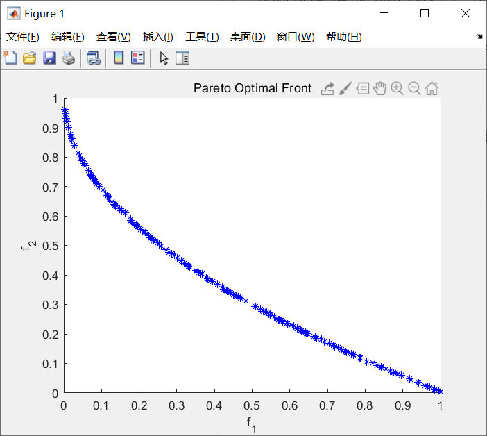
Figure 4-8 fitness function of nsga-2 algorithm
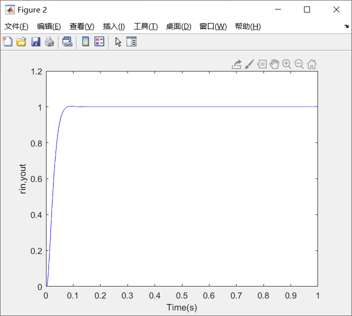
Figure 4-9 simulation results of PID parameter setting of nsga-2 algorithm
4 references
[1] Yuan Lei, Hu Bingxin, Wei keyin, et al Modern permanent magnet synchronous motor control principle and MATLAB simulation [M] Beijing: Beijing University of Aeronautics and Astronautics Press, 2016 (03): 12-18
[2]Deb K, Pratap A, Agarwal S, et al. A fast and elitist multiobjective genetic algorithm: NSGA-II[J]. IEEE Transactions on Evolutionary Computation, 2002, 6(2):182-197.
[3]Zhang Q, Li H. MOEA/D: A Multiobjective Evolutionary Algorithm Based on Decomposition[J]. IEEE Transactions on Evolutionary Computation, 2007, 11(6):712-731.
[4]M. Andersson, S. Bandaru and A. H. C. Ng, "Towards optimal algorithmic parameters for simulation-based multi-objective optimization," 2016 IEEE Congress on Evolutionary Computation (CEC), Vancouver, BC, 2016, pp. 5162-5169.