Source of this tutorial
The tutorial takes the model of automobile fuel efficiency as an example, with the number of cylinders, displacement, horsepower and weight as variables

Linear regression mathematical theory I learned before

get data

dataset_path = keras.utils.get_file("auto-mpg.data", "http://archive.ics.uci.edu/ml/machine-learning-databases/auto-mpg/auto-mpg.data")
# Not with keras datasets. A database. This is to read the file path for the following pandas
print(dataset_path) # At C: \ users \ wquiet \ keras\datasets\auto-mpg. data

# enumeration
column_names = ['MPG','Cylinders','Displacement','Horsepower','Weight',
                'Acceleration', 'Model Year', 'Origin']
raw_dataset = pd.read_csv(dataset_path, names=column_names,
                      na_values = "?", comment='\t',
                      sep=" ", skipinitialspace=True)

The first step of using pandas for data processing is to read data. Data sources can come from various places, and csv file is one of them. Pandas also provides very strong support for reading csv files, with 40 or 50 parameters.

1. Data input path: it can be a file path, a URL, or any object that implements the read method.
2. names: header, which is similar to ["number", "name", "address"]
3. na_values: here is to replace the question mark with NaN. The complete is {"a specified column": ["the content of that column to be replaced", "use brackets for more than 2"], "result": ["right"]})
4. sep: the separator specified when reading csv files. The default is comma. Note: "the separator of csv file" and "the separator specified when we read csv file" must be consistent.
   Explain pandas read in detail_ CSV method

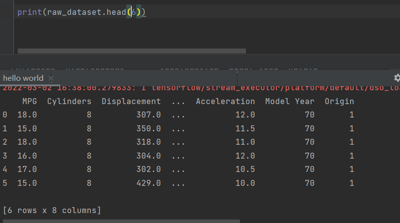
The following figure shows the raw data obtained

data processing

dataset = raw_dataset.copy() # Back up original data
print(dataset.isna().sum()) # Sum up the position count that is the vacancy value
dataset = dataset.dropna()# Remove the data with vacancy value in that row

origin = dataset.pop('Origin')
# The data in the "Origin" column represents countries, and the three countries are numbered 1, 2 and 3 respectively. But that classification is not intuitive, so it is divided into three columns, and only one country can set one [that is, one hot code]
dataset['USA'] = (origin == 1)*1.0
dataset['Europe'] = (origin == 2)*1.0
dataset['Japan'] = (origin == 3)*1.0

# Separate training set and test set
train_dataset = dataset.sample(frac=0.8,random_state=0)
test_dataset = dataset.drop(train_dataset.index)

DataFrame.sample(n=None, frac=None, replace=False, weights=None, random_state=None, axis=None)
(the number of rows to be extracted and the proportion of rows to be extracted [e.g. frac=0.8, that is, 80% of them to be extracted], whether it is put back sampling, I don't understand, can the data be repeated, choose the row or column to extract the data)
pandas.DataFrame.sample randomly selects several rows

View data content with data graph

sns.pairplot(train_dataset[["MPG", "Cylinders", "Displacement", "Weight"]], diag_kind="kde")

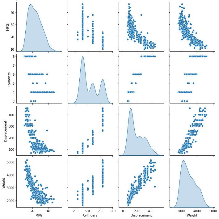
Seaborn is a Python visualization Library Based on matplotlib. It provides an advanced interface to draw attractive statistical graphics.
pairplot mainly shows the relationship between two variables
sns.pairplot(data,kind="reg",diag_kind="kde")
kind: used to control the type of graph on non diagonal lines. Options include "scatter" and "reg"
diag_kind: controls the type of graph on the diagonal. Options include "hist" and "kde"
Python visualization | Seaborn 5-minute Introduction (VII) -- pairplot
If the data chart is not displayed, add a PLT In the following header file of show(), import matplotlib pyplot as plt

View data content with table

train_stats = train_dataset.describe()
train_stats.pop("MPG") # Remove this column of data
train_stats = train_stats.transpose() # Matrix transpose is to interchange the labels of rows and columns
print(train_stats)

The describe () function can view the statistics of data in the DataFrame
Basic introduction to describe function
Detailed explanation of the parameters of the describe function of pandas

# Save the required data separately
train_labels = train_dataset.pop('MPG')
test_labels = test_dataset.pop('MPG')

# Normalize the data
def norm(x):
  return (x - train_stats['mean']) / train_stats['std']  # Here is the list after transpose... So this data type can only take one row, not one column?
normed_train_data = norm(train_dataset)
normed_test_data = norm(test_dataset)

Build model

def build_model():
  model = keras.Sequential([
    layers.Dense(64, activation='relu', input_shape=[len(train_dataset.keys())]),
    layers.Dense(64, activation='relu'),
    layers.Dense(1)
  ])

  optimizer = tf.keras.optimizers.RMSprop(0.001)

  model.compile(loss='mse',
                optimizer=optimizer,
                metrics=['mae', 'mse'])
  return model

model = build_model() # structure
model.summary() # Look at the details of the model

Training model

Suppose you have a dataset containing 200 samples (data rows) and you select a Batch size of 5 and 1000 Epoch.
This means that the dataset will be divided into 40 batches with 5 samples per Batch. After each Batch of five samples, the model weight will be updated.
This also means that an epoch will involve 40 batches or 40 model updates.
With 1000 epochs, the model will expose or deliver the entire data set 1000 times. There are a total of 40000 in the whole training process.
What is the difference between Batch and Epoch in neural network?
wq: so if you want to train faster, increase the batch or decrease the Epoch

Try it first

example_batch = normed_train_data[:10]
example_result = model.predict(example_batch)

predict generates an output forecast for the input sample. Just run the prediction with the newly built network and its initial parameters
There are predict and fit of model in the Chinese document

# The training progress is displayed by printing a point for each completed period
class PrintDot(keras.callbacks.Callback):
  def on_epoch_end(self, epoch, logs):
    if epoch % 100 == 0: print('')
    print('.', end='')

EPOCHS = 1000

history = model.fit(
  normed_train_data, train_labels,
  epochs=EPOCHS, validation_split = 0.2, verbose=0,
  callbacks=[PrintDot()])

The callback function, callback, is of type obj. He can let the model fit and is often called at various points. It can store the state of the model, take measures to interrupt the training, save the model, load different weights, or replace the state of the model.
Although we call it a callback "function", in fact, the callback function of Keras is a class. Defining a new callback function must inherit from this class
The callback function takes the dictionary logs as the parameter, which contains a series of information related to the current batch or epoch
At present, the model is The following parameters in fit() will be recorded in logs:

• At the end of each epoch (on_epoch_end), logs will contain the training accuracy and error, acc and loss. If a verification set is specified, it will also include the verification set accuracy and error val_acc) and val_loss，val_acc also needs to be added in Enable metrics = ['accuracy'] in compile.
• At the beginning of each batch (on_batch_begin): logs contains size, that is, the number of samples of the current batch
• At the end of each batch (on_batch_end): logs contains loss, and acc if accuracy is enabled
  Detailed explanation of callback function Callbacks in Keras

# The call is the same as above. The callback function is written to play
class PrintDot(keras.callbacks.Callback):
  def on_epoch_end(self, epoch, logs):
    if epoch % 10 == 0:print('a')
    print('n', end='b')
    print(logs)
  def on_batch_begin(self, batch, logs):
    if batch % 5 == 0:
        print('')
        print('2')
    print('3', end='c')

View data

def plot_history(history):
    # Basic steps of getting data
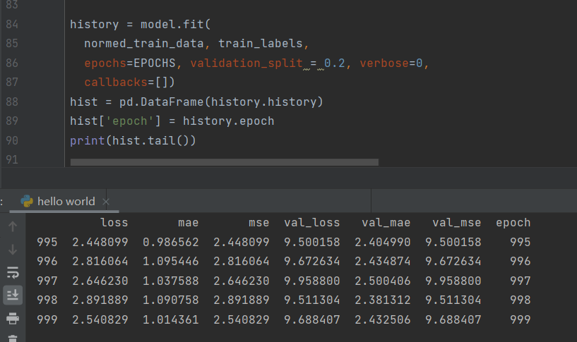
  hist = pd.DataFrame(history.history)
  hist['epoch'] = history.epoch

  plt.figure()# canvas
  plt.xlabel('Epoch')
  plt.ylabel('Mean Abs Error [MPG]')
  plt.plot(hist['epoch'], hist['mae'],# Draw lines according to data
           label='Train Error')
  plt.plot(hist['epoch'], hist['val_mae'],# It changes color automatically
           label = 'Val Error')
  plt.ylim([0,5])
  plt.legend()# Add the legend in the upper right corner

  plt.figure()
  plt.xlabel('Epoch')
  plt.ylabel('Mean Square Error [$MPG^2$]')
  plt.plot(hist['epoch'], hist['mse'],
           label='Train Error')
  plt.plot(hist['epoch'], hist['val_mse'],
           label = 'Val Error')
  plt.ylim([0,20])
  plt.legend()
  plt.show()


plot_history(history)

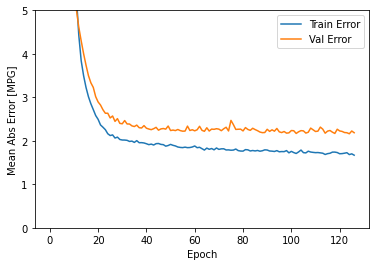
The data in the figure shows that the error of the training set is less and less, but the error of the test set is more and more large, which is probably over fitting.

Remedy model

In fact, add a callback to stop the model when the error of the training set is a little unreasonable.

model = build_model()

# The patience value is used to check the number of improved epochs
early_stop = keras.callbacks.EarlyStopping(monitor='val_loss', patience=10)

history = model.fit(normed_train_data, train_labels, epochs=EPOCHS,
                    validation_split = 0.2, verbose=0, callbacks=[early_stop, PrintDot()])

early_stop = keras.callbacks.EarlyStopping(monitor='val_loss',patience=50)

monitor: data interface for monitoring.
keras defines the following data interfaces that can be used directly:

• acc (accuracy), accuracy of test set
• Loss, loss function of test set (error)
• val_acc (val_accuracy) to verify the accuracy of the set
• val_loss, the loss function (error) of the verification set, which is the most commonly used monitoring interface, because monitoring the test set usually does not make much sense, and the loss function on the verification set is more meaningful.

Patient: for the set monitor, you can tolerate no improvement in how many epoch s. The patient should not be set too small to prevent premature stop of training due to early jitter. Of course, it should not be set too large, which will lose the meaning of EarlyStopping.

then
Take the test set and try it out

loss, mae, mse = model.evaluate(normed_test_data, test_labels, verbose=2)
print("Testing set Mean Abs Error: {:5.2f} MPG".format(mae))

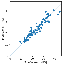
Make predictions

test_predictions = model.predict(normed_test_data).flatten()

plt.scatter(test_labels, test_predictions)
plt.xlabel('True Values [MPG]')
plt.ylabel('Predictions [MPG]')
plt.axis('equal')
plt.axis('square')
plt.xlim([0,plt.xlim()[1]])
plt.ylim([0,plt.ylim()[1]])
_ = plt.plot([-100, 100], [-100, 100])


# Error distribution
error = test_predictions - test_labels
plt.hist(error, bins = 25)
plt.xlabel("Prediction Error [MPG]")
_ = plt.ylabel("Count")

For example, we randomly define a data a with dimension (2, 3, 4). The effect of flatten() is the same as that of flatten(0). The data of a is expanded from 0 dimension, that is (2 * 3 * 4), and the length is (24). A expand flatten(1) from one dimension, that is, (2,3 * 4), that is, (2,12)
Detailed explanation of flatten() parameters

Code backup

Over fitting

import pathlib

import matplotlib.pyplot as plt
import pandas as pd
import seaborn as sns

import tensorflow as tf

from tensorflow import keras
from tensorflow.keras import layers

dataset_path = keras.utils.get_file("auto-mpg.data", "http://archive.ics.uci.edu/ml/machine-learning-databases/auto-mpg/auto-mpg.data")

column_names = ['MPG','Cylinders','Displacement','Horsepower','Weight',
                'Acceleration', 'Model Year', 'Origin']
raw_dataset = pd.read_csv(dataset_path, names=column_names,
                      na_values = "?", comment='\t',
                      sep=" ", skipinitialspace=True)
dataset = raw_dataset.copy()
dataset = dataset.dropna()
# print(dataset.isna().sum())

origin = dataset.pop('Origin')
# The data in the "Origin" column represents the country. But that classification is not intuitive, so it is divided into three columns, and only one country can set one [that is, one hot code]
dataset['USA'] = (origin == 1)*1.0
dataset['Europe'] = (origin == 2)*1.0
dataset['Japan'] = (origin == 3)*1.0

# Separate training set and test set
train_dataset = dataset.sample(frac=0.8,random_state=0)
test_dataset = dataset.drop(train_dataset.index)

# sns.pairplot(train_dataset[["MPG", "Cylinders", "Displacement", "Weight"]], diag_kind="kde")
# plt.show()
train_stats = train_dataset.describe()
train_stats.pop("MPG") # Remove this column of data
train_stats = train_stats.transpose() # Matrix transpose is to interchange the labels of rows and columns
# print(train_stats)

train_labels = train_dataset.pop('MPG')
test_labels = test_dataset.pop('MPG')

def norm(x):
  return (x - train_stats['mean']) / train_stats['std']
normed_train_data = norm(train_dataset)
normed_test_data = norm(test_dataset)
def build_model():
  model = keras.Sequential([
    layers.Dense(64, activation='relu', input_shape=[len(train_dataset.keys())]),
    layers.Dense(64, activation='relu'),
    layers.Dense(1)
  ])

  optimizer = tf.keras.optimizers.RMSprop(0.001)

  model.compile(loss='mse',
                optimizer=optimizer,
                metrics=['mae', 'mse'])
  return model
model = build_model()
# example_batch = normed_train_data[:10]
# example_result = model.predict(example_batch)
# print(example_result)

# The training progress is displayed by printing a point for each completed period
class PrintDot(keras.callbacks.Callback):
  def on_epoch_end(self, epoch, logs):
    if epoch % 10 == 0:print('a')
    print(logs)
#   def on_batch_begin(self, batch, logs):
#     if batch % 5 == 0:
#         print('')
#         print('2')
#     print('3', end='c')

# on_epoch_begin: it will be called automatically at the beginning of each epoch
# on_batch_begin: called at the beginning of each batch
# on_train_begin: called at the beginning of training
# on_train_end: called at the end of training

EPOCHS = 100

history = model.fit(
  normed_train_data, train_labels,
  epochs=EPOCHS, validation_split = 0.2, verbose=0,
  callbacks=[PrintDot()])
hist = pd.DataFrame(history.history)
hist['epoch'] = history.epoch
print(hist.tail())


def plot_history(history):
    # Basic steps of getting data
  hist = pd.DataFrame(history.history)
  hist['epoch'] = history.epoch

  plt.figure()# canvas
  plt.xlabel('Epoch')
  plt.ylabel('Mean Abs Error [MPG]')
  plt.plot(hist['epoch'], hist['mae'],# Draw lines according to data
           label='Train Error')
  plt.plot(hist['epoch'], hist['val_mae'],# It changes color automatically
           label = 'Val Error')
  plt.ylim([0,5])
  plt.legend()# Add the legend in the upper right corner

  plt.figure()
  plt.xlabel('Epoch')
  plt.ylabel('Mean Square Error [$MPG^2$]')
  plt.plot(hist['epoch'], hist['mse'],
           label='Train Error')
  plt.plot(hist['epoch'], hist['val_mse'],
           label = 'Val Error')
  plt.ylim([0,20])
  plt.legend()
  plt.show()


plot_history(history)

Well sorted out the code

import pathlib

import matplotlib.pyplot as plt
import pandas as pd
import seaborn as sns

import tensorflow as tf

from tensorflow import keras
from tensorflow.keras import layers

# Build model
def build_model():
  model = keras.Sequential([
    layers.Dense(64, activation='relu', input_shape=[len(train_dataset.keys())]),
    layers.Dense(64, activation='relu'),
    layers.Dense(1)
  ])

  optimizer = tf.keras.optimizers.RMSprop(0.001)

  model.compile(loss='mse',
                optimizer=optimizer,
                metrics=['mae', 'mse'])
  return model

# Callback
# The training progress is displayed by printing a point for each completed period
class PrintDot(keras.callbacks.Callback):
  def on_epoch_end(self, epoch, logs):
    if epoch % 10 == 0:print('a')
    print(logs)
#   def on_batch_begin(self, batch, logs):
#     if batch % 5 == 0:
#         print('')
#         print('2')
#     print('3', end='c')

# on_epoch_begin: it will be called automatically at the beginning of each epoch
# on_batch_begin: called at the beginning of each batch
# on_train_begin: called at the beginning of training
# on_train_end: called at the end of training

# Show the variation diagram of error epoch
def plot_history(history):
    # Basic steps of getting data
  hist = pd.DataFrame(history.history)
  hist['epoch'] = history.epoch

  plt.figure()# canvas
  plt.xlabel('Epoch')
  plt.ylabel('Mean Abs Error [MPG]')
  plt.plot(hist['epoch'], hist['mae'],# Draw lines according to data
           label='Train Error')
  plt.plot(hist['epoch'], hist['val_mae'],# It changes color automatically
           label = 'Val Error')
  plt.ylim([0,5])
  plt.legend()# Add the legend in the upper right corner

  plt.figure()
  plt.xlabel('Epoch')
  plt.ylabel('Mean Square Error [$MPG^2$]')
  plt.plot(hist['epoch'], hist['mse'],
           label='Train Error')
  plt.plot(hist['epoch'], hist['val_mse'],
           label = 'Val Error')
  plt.ylim([0,20])
  plt.legend()
  plt.show()


# Extract data path
dataset_path = keras.utils.get_file("auto-mpg.data", "http://archive.ics.uci.edu/ml/machine-learning-databases/auto-mpg/auto-mpg.data")
#Enumeration specifies the meaning of the data
column_names = ['MPG','Cylinders','Displacement','Horsepower','Weight',
                'Acceleration', 'Model Year', 'Origin']
# Save data
raw_dataset = pd.read_csv(dataset_path, names=column_names,
                      na_values = "?", comment='\t',
                      sep=" ", skipinitialspace=True)
# Backup data
dataset = raw_dataset.copy()
dataset = dataset.dropna()# Discard those rows with data gaps
# print(dataset.isna().sum())

origin = dataset.pop('Origin')
# The data in the "Origin" column represents the country. But that classification is not intuitive, so it is divided into three columns, and only one country can set one [that is, one hot code]
dataset['USA'] = (origin == 1)*1.0
dataset['Europe'] = (origin == 2)*1.0
dataset['Japan'] = (origin == 3)*1.0

# Separate training set and test set
train_dataset = dataset.sample(frac=0.8,random_state=0)# Take 80% of the data randomly and without repetition
test_dataset = dataset.drop(train_dataset.index) # Test set = source data set - training set

# sns.pairplot(train_dataset[["MPG", "Cylinders", "Displacement", "Weight"]], diag_kind="kde")
# plt.show()

train_stats = train_dataset.describe()# Obtain data statistical results
train_stats.pop("MPG") # Remove this column of data
train_stats = train_stats.transpose() # Matrix transpose is to interchange the labels of rows and columns
# print(train_stats)

train_labels = train_dataset.pop('MPG')# Train_ The column of data in the dataset is stored in the train_labels
test_labels = test_dataset.pop('MPG')

# data normalization 
def norm(x):
  return (x - train_stats['mean']) / train_stats['std']
normed_train_data = norm(train_dataset)
normed_test_data = norm(test_dataset)

# Build model
model = build_model()
# print(model.summary()) #Check model
# Trial prediction
# example_batch = normed_train_data[:10]
# example_result = model.predict(example_batch)
# print(example_result)

# Training the model in EPOCHS cycles [this database has to be trained EPOCHS times
EPOCHS = 100

# Monitor the loss function (error) of the verification set. Stop training if continuous patience data are getting worse and worse
early_stop = keras.callbacks.EarlyStopping(monitor='val_loss', patience=50)
# Train and save historical data
history = model.fit(
  normed_train_data, train_labels,
  epochs=EPOCHS, validation_split = 0.2, verbose=0,
  callbacks=[early_stop, PrintDot()])


# Show loss Mae MSE Val in a table_ loss val_ mae val_ MSE epoch and other data
# hist = pd.DataFrame(history.history)
# hist['epoch'] = history.epoch # Take epoch as the number of rows
# print(hist.tail())

# Show the change of error -epoch with a graph
# plot_history(history)

# Test set commissioning model
loss, mae, mse = model.evaluate(normed_test_data, test_labels, verbose=2)
print("Testing set Mean Abs Error: {:5.2f} MPG".format(mae))# mpg is an American unit of fuel consumption

# Predict and reduce the output data to 1 dimension
test_predictions = model.predict(normed_test_data).flatten()
# flatten() is a dimension reduction function for multidimensional data.

# Use the data in the test set to predict the MPG value:
plt.scatter(test_labels, test_predictions)
plt.xlabel('True Values [MPG]')
plt.ylabel('Predictions [MPG]')
plt.axis('equal')
plt.axis('square')
plt.xlim([0,plt.xlim()[1]])
plt.ylim([0,plt.ylim()[1]])
_ = plt.plot([-100, 100], [-100, 100])
plt.show()

# Look at the error distribution
error = test_predictions - test_labels
plt.hist(error, bins = 25)
plt.xlabel("Prediction Error [MPG]")
_ = plt.ylabel("Count")
plt.show()