reference:
https://zhuanlan.zhihu.com/p/71328244
catalogue
It's true that you have to pay it back sooner or later. You've always refused to learn Tensorboard because there are alternatives until you find that you have to use it. The following mainly introduces how to use Tensorboard to visualize variables such as parameters, loss and accuracy.
1. Visual calculation diagram
The following is an example of handwriting classification of a single-layer network:
import tensorflow as tf
from tensorflow.examples.tutorials.mnist import input_data

mnist = input_data.read_data_sets("MNIST_data", one_hot=True)

batch_size = 100
n_batch = mnist.train.num_examples // batch_size

with tf.name_scope('input'):
    x = tf.placeholder(dtype=tf.float32, shape=[None, 784], name='x_input')
    y = tf.placeholder(dtype=tf.int32, shape=[None, 10], name='y_input')

with tf.name_scope('layer'):
    with tf.name_scope('weights'):
        W = tf.Variable(tf.random_uniform([784, 10]), name='w')
    with tf.name_scope('biases'):
        b = tf.Variable(tf.zeros(shape=[10], dtype=tf.float32), name='b')
    with tf.name_scope('softmax'):
        prediction = tf.nn.softmax(tf.nn.xw_plus_b(x, W, b))
with tf.name_scope('Loss'):
    loss = tf.reduce_mean(tf.nn.softmax_cross_entropy_with_logits(labels=y, logits=prediction))
with tf.name_scope('train'):
    train_step = tf.train.GradientDescentOptimizer(0.01).minimize(loss)
with tf.name_scope('acc'):
    correct_prediction = tf.equal(tf.argmax(y, 1), tf.argmax(prediction, 1))
    acc = tf.reduce_mean(tf.cast(correct_prediction, tf.float32))

with tf.Session() as sess:
    sess.run(tf.global_variables_initializer())
    writer = tf.summary.FileWriter('logs/', sess.graph)
    for epoch in range(20):
        for batch in range(n_batch):
            batch_x, batch_y = mnist.train.next_batch(batch_size)
            _, accuracy = sess.run([train_step, acc], feed_dict={x: batch_x, y: batch_y})
            if batch % 50 == 0:
                print("### Epoch: {}, batch: {} acc on train: {}".format(epoch, batch, accuracy))
        accuracy = sess.run(acc, feed_dict={x: mnist.test.images, y: mnist.test.labels})
        print("### Epoch: {},  acc on test: {}".format(epoch, accuracy))
The visualization results of the calculation diagram are as follows:
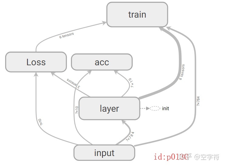
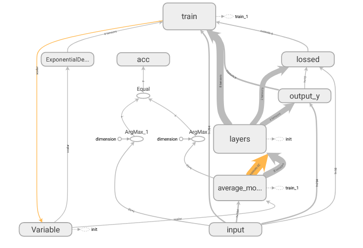
The gray rounded rectangle in the figure is the namespace TF in the code name_ Scope (), and namespaces can be nested and defined. From the calculation diagram, you can clearly see the details of each operation, as well as the shape and flow direction of the data volume. The implementation of this operation depends entirely on the code in line 31. After executing this code, a similar code named events. Will be generated in the path you specify (here is the logs folder of the path where the code is located) out. tfevents. 156171787. The opening steps are as follows:
- First, you need to install tensorflow and tensorboard;
- Open the command line (Linux terminal) and enter the upper directory of log;
- Run the command tensorboard --logdir=logs
- If successful, the following prompt will appear:
- TensorBoard 1.5.1 at http://DESKTOP-70LJI62:6006 (Press CTRL+C to quit)
- If there is any error, the most direct way is to uninstall tensorflow and reinstall it. If there are multiple environments, Anaconda management is recommended
- Paste the following address into the browser (preferably Google), and then you can see it. You can double-click each node to view the details
2. Visual parameters
The visual network calculation diagram is not very meaningful, but it is more meaningful to see the transformation curve of some parameters (such as accuracy, loss, etc.) while training the network, so as to better analyze the network.
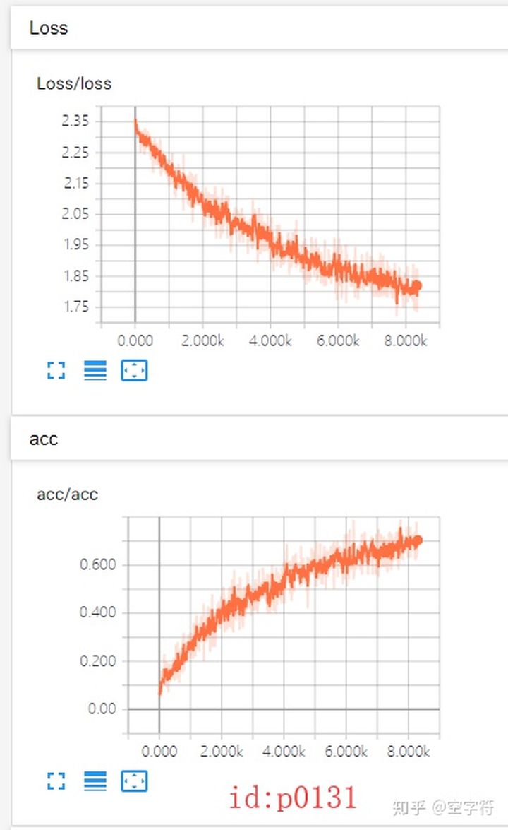
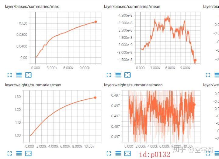
To implement this operation, you only need to add the corresponding TF summary. Scalar ('acc ', ACC) statement, and then merge all the summaries. However, generally, the parameters of the network layer are not scalars, but matrices; For this kind of variable, the usual method is to calculate its maximum, minimum, average and histogram. Since the same operations are used for many parameters, the functions are uniformly defined here:
def variable_summaries(var):
    with tf.name_scope('summaries'):
        mean = tf.reduce_mean(var)
        tf.summary.scalar('mean', mean)
        with tf.name_scope('stddev'):
            stddev = tf.sqrt(tf.reduce_mean(tf.square(var - mean)))
        tf.summary.scalar('stddev', stddev)
        tf.summary.scalar('max', tf.reduce_max(var))
        tf.summary.scalar('min', tf.reduce_min(var))
        tf.summary.histogram('histogram', var)
Then call this function where you need visual parameters.
mnist = input_data.read_data_sets("MNIST_data", one_hot=True)

batch_size = 100

n_batch = mnist.train.num_examples // batch_size
with tf.name_scope('input'):
    x = tf.placeholder(dtype=tf.float32, shape=[None, 784], name='x_input')
    y = tf.placeholder(dtype=tf.int32, shape=[None, 10], name='y_input')

with tf.name_scope('layer'):
    with tf.name_scope('weights'):
        W = tf.Variable(tf.random_uniform([784, 10]), name='w')
        variable_summaries(W)####
    with tf.name_scope('biases'):
        b = tf.Variable(tf.zeros(shape=[10], dtype=tf.float32), name='b')
        variable_summaries(b)
    with tf.name_scope('softmax'):
        prediction = tf.nn.softmax(tf.nn.xw_plus_b(x, W, b))
with tf.name_scope('Loss'):
    loss = tf.reduce_mean(tf.nn.softmax_cross_entropy_with_logits(labels=y, logits=prediction))
    tf.summary.scalar('loss', loss)
with tf.name_scope('train'):
    train_step = tf.train.GradientDescentOptimizer(0.01).minimize(loss)
with tf.name_scope('acc'):
    correct_prediction = tf.equal(tf.argmax(y, 1), tf.argmax(prediction, 1))
    acc = tf.reduce_mean(tf.cast(correct_prediction, tf.float32))
    tf.summary.scalar('acc', acc)

merged = tf.summary.merge_all()
with tf.Session() as sess:
    sess.run(tf.global_variables_initializer())
    writer = tf.summary.FileWriter('logs/', sess.graph)
    for epoch in range(20):
        for batch in range(n_batch):
            batch_x, batch_y = mnist.train.next_batch(batch_size)
            _, summary, accuracy = sess.run([train_step, merged, acc], feed_dict={x: batch_x, y: batch_y})
            if batch % 50 == 0:
                print("### Epoch: {}, batch: {} acc on train: {}".format(epoch, batch, accuracy))
            writer.add_summary(summary, epoch * n_batch + batch)
        accuracy = sess.run(acc, feed_dict={x: mnist.test.images, y: mnist.test.labels})
        print("### Epoch: {},  acc on test: {}".format(epoch, accuracy))
As shown in lines 14, 17, 22 and 28 of the above code. Finally, at each iteration, the merged is calculated and written in the local file (line 40). Finally, according to the above method, open it with tensorboard.
Note: this can be visualized without waiting for the whole training process, but you can see it during the training process. It is Nice to refresh it every 30 seconds according to the generated data.
3. Remote tensorboard
Due to the limited conditions, the training is usually carried out on a remote server during in-depth learning, so how to visualize it on the local computer at this time? The answer is to use the direction tunnel technology of SSH to forward the port data on the server to the corresponding local port, and then the log data on the local method server can be.
From the above prompt after successful connection, we can know that the port used by tensorboard is 6006 (it may be changed one day), so we just need to forward the data of this port to the local.
- ssh -L 16006:127.0.0.1:6006 account@server.address
- 16006 is any local port, which can be written freely as long as it does not conflict with the local application;
- The following account refers to the user name of your server, followed by Ip
For windows, just execute this command directly on the command line (I don't know when the windows command line also supports ssh)
After successful login (the server has been logged in remotely at this time), also enter the upper directory of logs directory, and then run tensorboard --logdir=logs; Finally, run 127.0.0.1:16006 in the local browser.
4. Error reporting
"AttributeError: module 'tensorflow' has no attribute 'io'" error may appear
This may be because the version of tensorboard is too high or does not match the version of tensorflow
My tensorflow version is 1.5.0 and tensorboard version is 1.8.0. Finally, I solved the error reporting