
Author: Han Xinzi@ShowMeAI
Tutorial address: http://www.showmeai.tech/tutorials/84
Article address: http://www.showmeai.tech/article-detail/181
Notice: All Rights Reserved. Please contact the platform and the author for reprint and indicate the source
1. Classification, regression and clustering model
1) Overview of classification algorithm
Classification is an important technology of machine learning and data mining. The purpose of classification is to construct a classification function or classification model (often called classifier) according to the characteristics of data set. The model can map the samples of unknown categories to a technology in a given category.
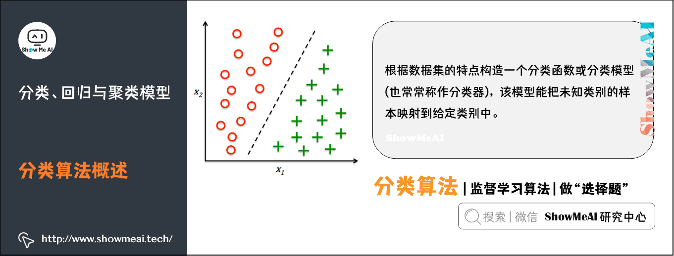
The purpose of classification is to analyze the input data, find an accurate description or model for each class through the characteristics of the data in the training set, and use this method (model) to express the implicit function.
The process of constructing classification model is generally divided into two stages: training and testing.
- Before constructing the model, the data set is randomly divided into training data set and test data set.
- Firstly, the training data set is used to construct the classification model, and then the test data set is used to evaluate the classification accuracy of the model.
- If the accuracy of the model is considered acceptable, the model can be used to classify other data tuples.
Generally speaking, the cost of the testing phase is much lower than that of the training phase.
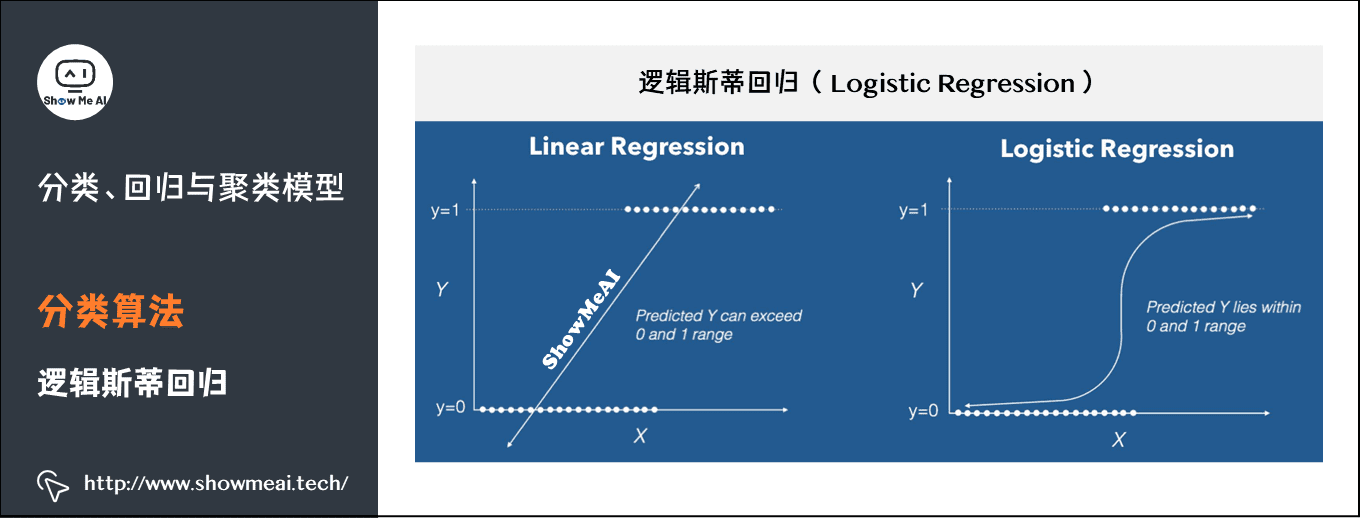
(1) Logistic regression
Logistic regression is a classical classification method in statistical learning, which belongs to log linear model. The dependent variables of logistic regression can be dichotomous or multiclassical.
- Get data set and code → official GitHub of ShowMeAI https://github.com/ShowMeAI-Hub/awesome-AI-cheatsheets
- Running code segment and learning → online programming environment http://blog.showmeai.tech/python3-compiler
from pyspark.ml.classification import LogisticRegression
from pyspark.sql import SparkSession

spark = SparkSession \
    .builder \
    .appName("LogisticRegressionSummary") \
    .getOrCreate()

# Load data
training = spark.read.format("libsvm").load("data/mllib/sample_libsvm_data.txt")

lr = LogisticRegression(maxIter=10, regParam=0.3, elasticNetParam=0.8)

# Fitting model
lrModel = lr.fit(training)

# Model information summary and output
trainingSummary = lrModel.summary

# Output the loss function value of each round
objectiveHistory = trainingSummary.objectiveHistory
print("objectiveHistory:")
for objective in objectiveHistory:
    print(objective)

# ROC curve
trainingSummary.roc.show()
print("areaUnderROC: " + str(trainingSummary.areaUnderROC))

spark.stop()
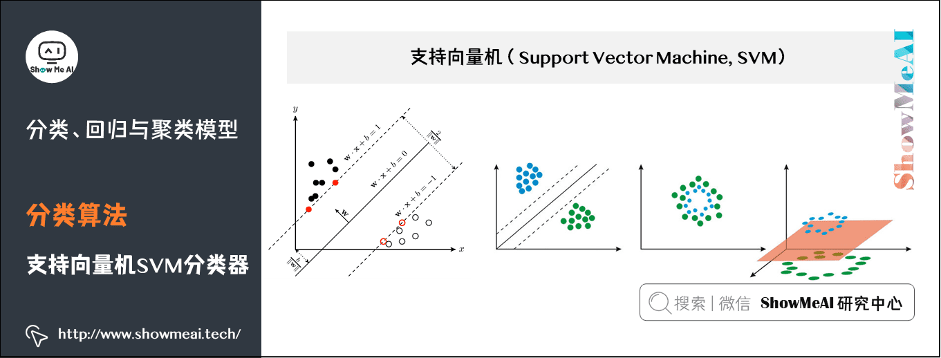
(2) Support vector machine SVM classifier
SVM is a support vector machine classification model. Its basic model is the linear classifier with the largest interval defined in the feature space. The learning method of support vector machine includes three models: linear separable support vector machine, linear support vector machine and nonlinear support vector machine.
- When the training data is linearly separable, a linear classifier, namely linear separable support vector machine, is learned by maximizing the hard interval;
- When the training data is approximately linearly separable, a linear classifier, namely linear support vector machine, is also learned by maximizing the soft interval;
- When the training data are linearly inseparable, the nonlinear support vector machine is learned by using kernel technique and soft interval maximization.
Linear support vector machines support regularized variants of L1 and L2.
- Get data set and code → official GitHub of ShowMeAI https://github.com/ShowMeAI-Hub/awesome-AI-cheatsheets
- Running code segment and learning → online programming environment http://blog.showmeai.tech/python3-compiler
from pyspark.ml.classification import LinearSVC

# Load training data
training = spark.read.format("libsvm").load("data/mllib/sample_libsvm_data.txt")

lsvc = LinearSVC(maxIter=10, regParam=0.1)

# Fit the model
lsvcModel = lsvc.fit(training)

# Print the coefficients and intercept for linear SVC
print("Coefficients: " + str(lsvcModel.coefficients))
print("Intercept: " + str(lsvcModel.intercept))
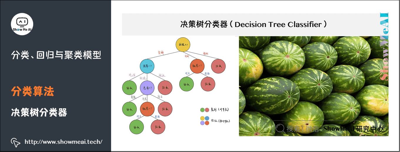
(3) Decision tree classifier
Decision tree is a basic classification and regression method. This paper mainly introduces the decision tree used for classification. The decision tree pattern is a tree structure, in which each internal node represents a test on an attribute, each branch represents a test output, and each leaf node represents a category.
When learning, the decision tree model is established according to the principle of minimizing the loss function by using the training data; When forecasting, the new data are classified by decision tree model.
- Get data set and code → official GitHub of ShowMeAI https://github.com/ShowMeAI-Hub/awesome-AI-cheatsheets
- Running code segment and learning → online programming environment http://blog.showmeai.tech/python3-compiler
from pyspark.ml import Pipeline
from pyspark.ml.classification import DecisionTreeClassifier
from pyspark.ml.feature import StringIndexer, VectorIndexer
from pyspark.ml.evaluation import MulticlassClassificationEvaluator

# Load the data stored in LIBSVM format as a DataFrame.
data = spark.read.format("libsvm").load("data/mllib/sample_libsvm_data.txt")

# Index labels, adding metadata to the label column.
# Fit on whole dataset to include all labels in index.
labelIndexer = StringIndexer(inputCol="label", outputCol="indexedLabel").fit(data)
# Automatically identify categorical features, and index them.
# We specify maxCategories so features with > 4 distinct values are treated as continuous.
featureIndexer =\
    VectorIndexer(inputCol="features", outputCol="indexedFeatures", maxCategories=4).fit(data)

# Split the data into training and test sets (30% held out for testing)
(trainingData, testData) = data.randomSplit([0.7, 0.3])

# Train a DecisionTree model.
dt = DecisionTreeClassifier(labelCol="indexedLabel", featuresCol="indexedFeatures")

# Chain indexers and tree in a Pipeline
pipeline = Pipeline(stages=[labelIndexer, featureIndexer, dt])

# Train model.  This also runs the indexers.
model = pipeline.fit(trainingData)

# Make predictions.
predictions = model.transform(testData)

# Select example rows to display.
predictions.select("prediction", "indexedLabel", "features").show(5)

# Select (prediction, true label) and compute test error
evaluator = MulticlassClassificationEvaluator(
    labelCol="indexedLabel", predictionCol="prediction", metricName="accuracy")
accuracy = evaluator.evaluate(predictions)
print("Test Error = %g " % (1.0 - accuracy))

treeModel = model.stages[2]
# summary only
print(treeModel)
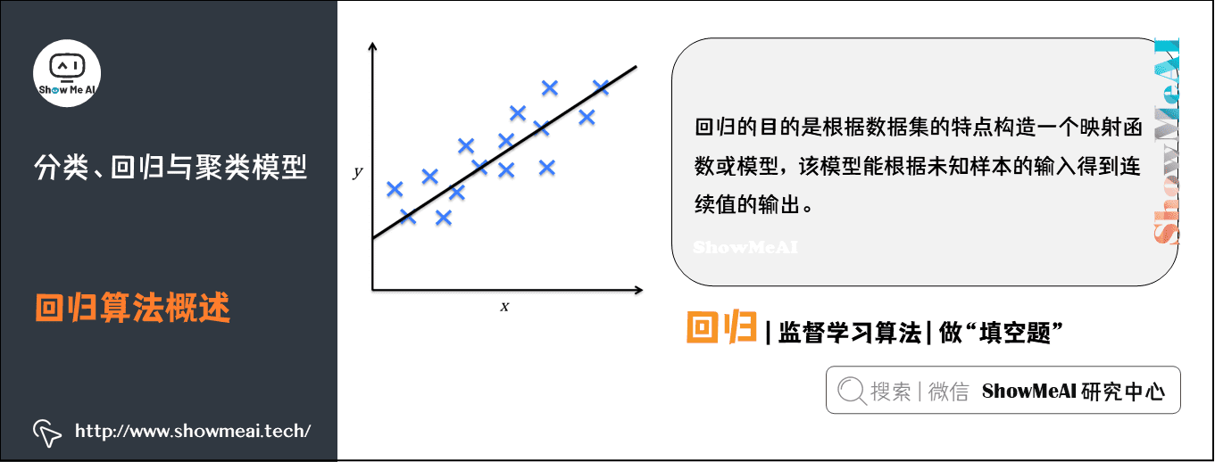
2) Overview of regression algorithm
Regression is also an important machine learning and data mining technology. The purpose of regression is to construct a mapping function or model according to the characteristics of the data set, which can obtain the output of continuous values according to the input of unknown samples.
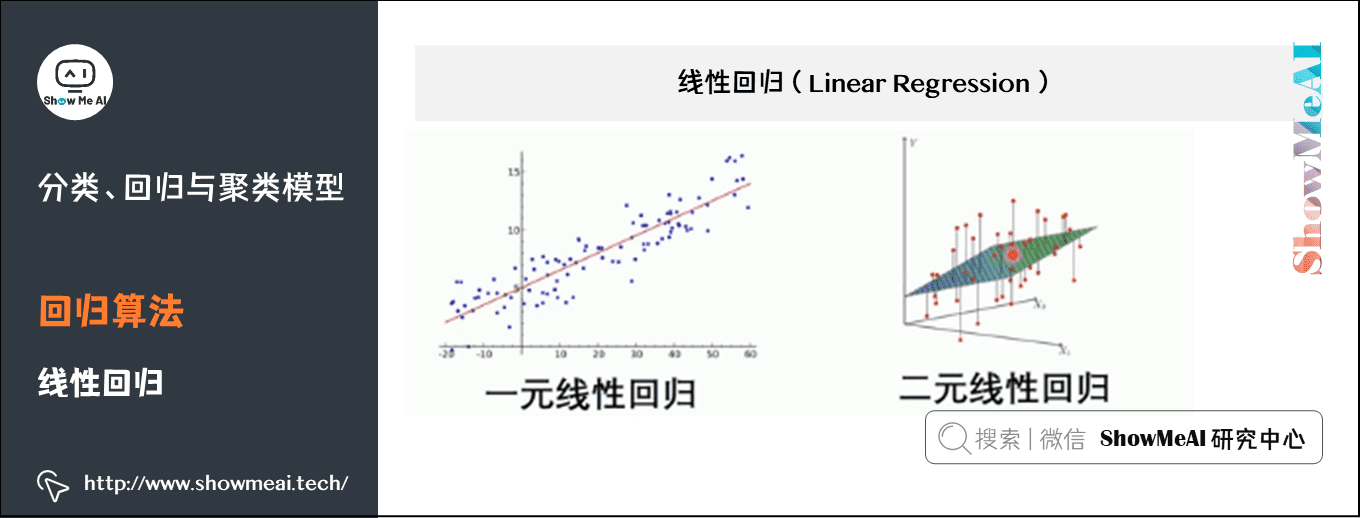
(1) Linear regression
Linear regression is a statistical analysis method that uses regression analysis in mathematical statistics to determine the interdependent quantitative relationship between two or more variables. It is widely used. The expression is y = w'x+e, e is the error, which follows the normal distribution with mean value of 0.
In regression analysis, only one independent variable and one dependent variable are included, and the relationship between them can be approximately expressed by a straight line. This regression analysis is called univariate linear regression analysis.
If the regression analysis includes two or more independent variables, and there is a linear relationship between dependent variables and independent variables, it is called multiple linear regression analysis.
- Get data set and code → official GitHub of ShowMeAI https://github.com/ShowMeAI-Hub/awesome-AI-cheatsheets
- Running code segment and learning → online programming environment http://blog.showmeai.tech/python3-compiler
from pyspark.ml.regression import LinearRegression

# Load training data
training = spark.read.format("libsvm")\
    .load("data/mllib/sample_linear_regression_data.txt")

lr = LinearRegression(maxIter=10, regParam=0.3, elasticNetParam=0.8)

# Fit the model
lrModel = lr.fit(training)

# Print the coefficients and intercept for linear regression
print("Coefficients: %s" % str(lrModel.coefficients))
print("Intercept: %s" % str(lrModel.intercept))

# Summarize the model over the training set and print out some metrics
trainingSummary = lrModel.summary
print("numIterations: %d" % trainingSummary.totalIterations)
print("objectiveHistory: %s" % str(trainingSummary.objectiveHistory))
trainingSummary.residuals.show()
print("RMSE: %f" % trainingSummary.rootMeanSquaredError)
print("r2: %f" % trainingSummary.r2)
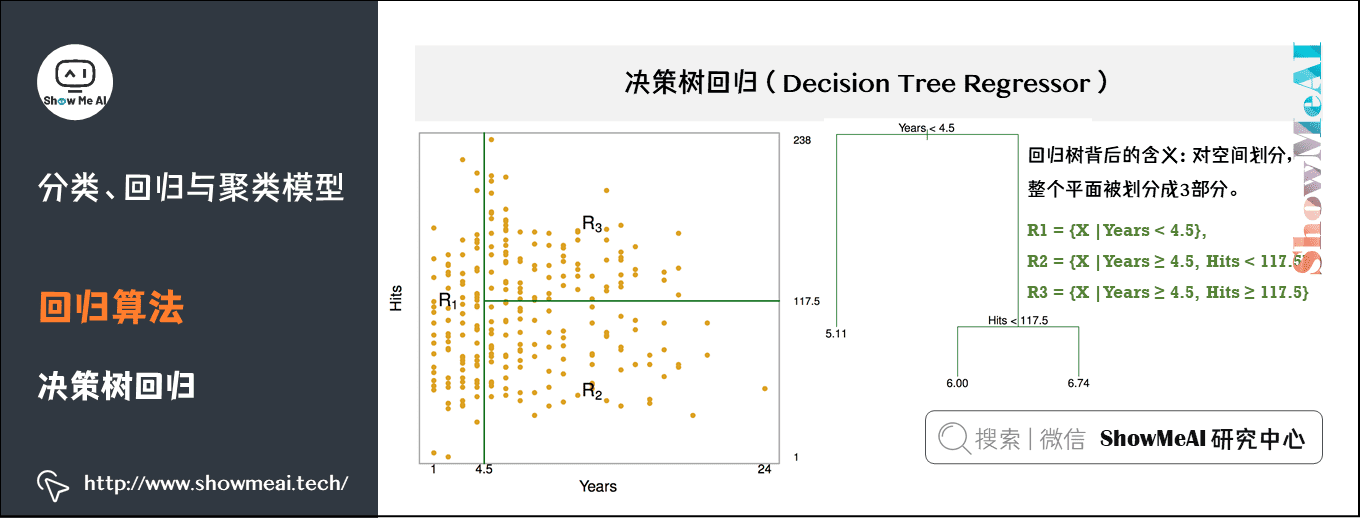
(2) Decision tree regression
The decision tree model can not only solve the classification problem (corresponding to the classification tree), that is, the corresponding target value is category data, but also be applied to the solution of regression prediction problem (regression tree), and its output value can be continuous real value.
Estimate the salary of baseball players according to their working years and performance. As shown in the figure, there are 1987 data samples, including 322 baseball players. Red and yellow indicate high income and blue and green indicate low income. The abscissa is the number of years and the ordinate is the expression.
- Get data set and code → official GitHub of ShowMeAI https://github.com/ShowMeAI-Hub/awesome-AI-cheatsheets
- Running code segment and learning → online programming environment http://blog.showmeai.tech/python3-compiler
from pyspark.ml import Pipeline
from pyspark.ml.regression import DecisionTreeRegressor
from pyspark.ml.feature import VectorIndexer
from pyspark.ml.evaluation import RegressionEvaluator
from pyspark.sql import SparkSession

spark = SparkSession\
    .builder\
    .appName("DecisionTreeRegressionExample")\
    .getOrCreate()

# Load data
data = spark.read.format("libsvm").load("data/mllib/sample_libsvm_data.txt")

# Automatically identify categorical features, and index them.
# We specify maxCategories so features with > 4 distinct values are treated as continuous.
featureIndexer =\
    VectorIndexer(inputCol="features", outputCol="indexedFeatures", maxCategories=4).fit(data)

# Split the data into training and test sets (30% held out for testing)
(trainingData, testData) = data.randomSplit([0.7, 0.3])

# Train a DecisionTree model.
dt = DecisionTreeRegressor(featuresCol="indexedFeatures")

# Chain indexer and tree in a Pipeline
pipeline = Pipeline(stages=[featureIndexer, dt])

# Train model.  This also runs the indexer.
model = pipeline.fit(trainingData)

# Make predictions.
predictions = model.transform(testData)

# Select example rows to display.
predictions.select("prediction", "label", "features").show(5)

# Select (prediction, true label) and compute test error
evaluator = RegressionEvaluator(
    labelCol="label", predictionCol="prediction", metricName="rmse")
rmse = evaluator.evaluate(predictions)
print("Root Mean Squared Error (RMSE) on test data = %g" % rmse)

treeModel = model.stages[1]
# summary only
print(treeModel)

spark.stop()
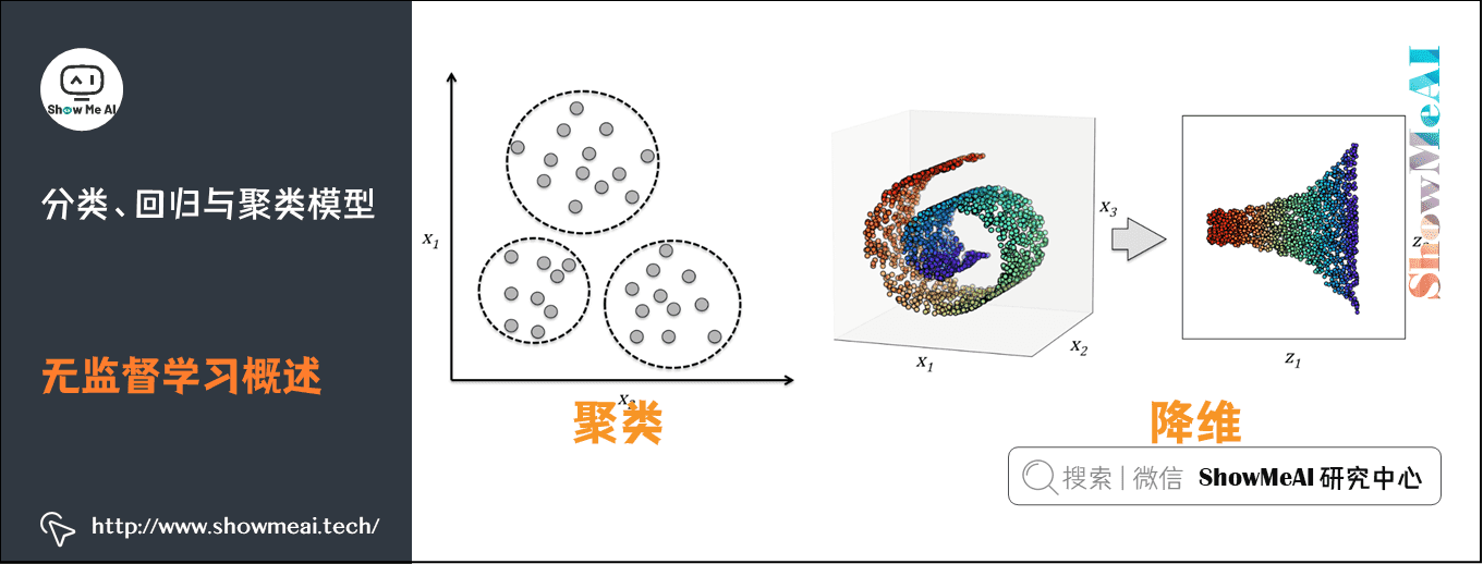
3) Overview of unsupervised learning
Using unlabeled data to learn the distribution of data or the relationship between data is called unsupervised learning.
- The biggest difference between supervised learning and unsupervised learning is whether the data has labels
- The most commonly used scenarios of unsupervised learning are clustering and dimension reduction
(1) Clustering algorithm
Clustering is an important method in machine learning. The main idea is to use different characteristic attributes of samples, find similar samples according to a given similarity measurement method (such as Euclidean distance), and divide the samples into different groups according to the distance. Clustering is a typical Unsupervised Learning method.
Compared with unsupervised learning (such as unsupervised learning set), unsupervised learning results. In unsupervised learning, data is not specially identified, and the learning model is to infer some internal structures of data.
Spark's MLlib library provides the implementation of many available clustering methods, such as K-Means, Gaussian mixture model, Power Iteration Clustering (PIC), implicit Dirichlet distribution (LDA), bisection K-Means and Streaming K-Means.
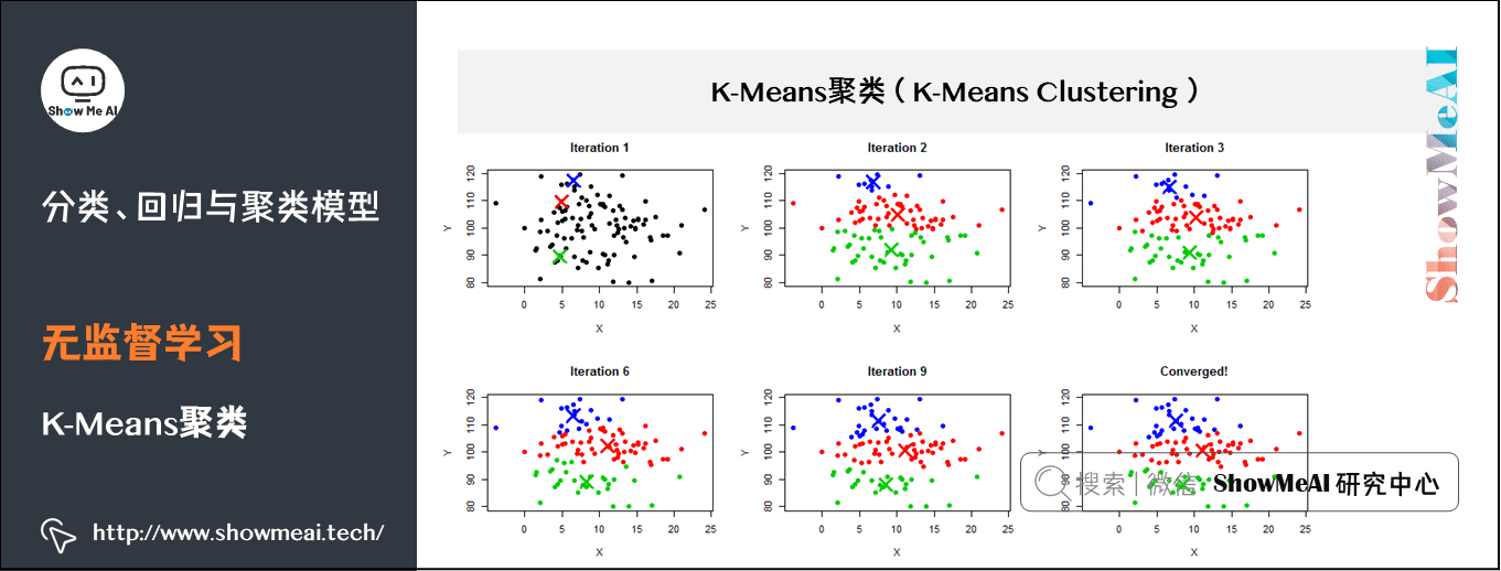
(2) K-Means clustering
K-Means is an iterative clustering algorithm, which belongs to the Partitioning clustering method, that is, first create K partitions, and then iteratively transfer samples from one partition to another to improve the quality of final clustering. The process of K-Means is roughly as follows:
- 1. Select k sample points as the initial division center according to the given K value;
- 2. Calculate the distance from all sample points to each division center, and divide all sample points to the nearest division center;
- 3. Calculate the average value of sample points in each division and take it as the new center;
- Cycle for 2 ~ 3 steps until the maximum number of iterations is reached, or the change of division center is less than a predefined threshold
- Get data set and code → official GitHub of ShowMeAI https://github.com/ShowMeAI-Hub/awesome-AI-cheatsheets
- Running code segment and learning → online programming environment http://blog.showmeai.tech/python3-compiler
spark = SparkSession\
        .builder\
        .appName("KMeansExample")\
        .getOrCreate()

dataset = spark.read.format("libsvm").load("data/mllib/sample_kmeans_data.txt")

# Training K-means clustering model
kmeans = KMeans().setK(2).setSeed(1)
model = kmeans.fit(dataset)

# Prediction (i.e. assigning cluster centers)
predictions = model.transform(dataset)

# According to the score of Silhouette (added in pyspark 2.2)
evaluator = ClusteringEvaluator()
silhouette = evaluator.evaluate(predictions)
print("Silhouette with squared euclidean distance = " + str(silhouette))

# Output prediction results
print("predicted Center: ")
for center in predictions[['prediction']].collect():
    print(center.asDict())

# Cluster center
centers = model.clusterCenters()
print("Cluster Centers: ")
for center in centers:
    print(center)

spark.stop()
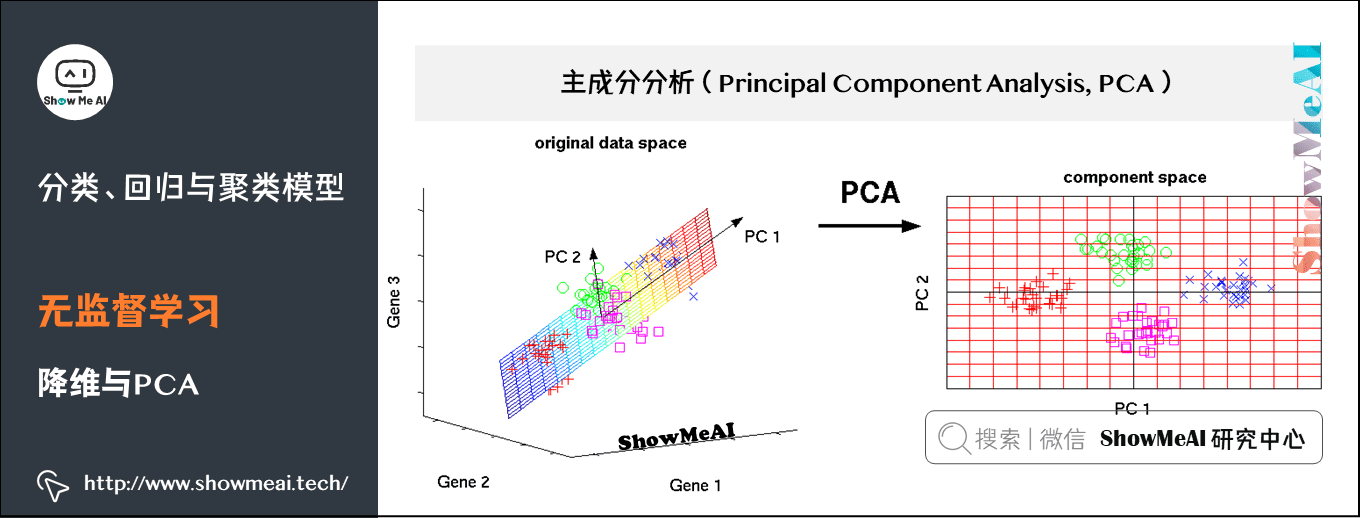
(3) Dimensionality reduction and PCA
Principal Component analysis (PCA) is a statistical method for data rotation transformation. Its essence is to carry out a base transformation in linear space to maximize the variance of the transformed data projected on a new set of "coordinate axes". Then, the "coordinate axes" with small variance after transformation are cut out, The remaining new "coordinate axes" are called principal components, which can represent the nature of the original data as much as possible in a lower dimensional subspace.
Principal component analysis is widely used in various statistics and machine learning problems. It is one of the most common dimensionality reduction methods.
- Get data set and code → official GitHub of ShowMeAI https://github.com/ShowMeAI-Hub/awesome-AI-cheatsheets
- Running code segment and learning → online programming environment http://blog.showmeai.tech/python3-compiler
spark = SparkSession\
        .builder\
        .appName("PCAExample")\
        .getOrCreate()

# Build a fake data
data = [(Vectors.sparse(5, [(1, 1.0), (3, 7.0)]),),
        (Vectors.dense([2.0, 0.0, 3.0, 4.0, 5.0]),),
        (Vectors.dense([4.0, 0.0, 0.0, 6.0, 7.0]),)]
df = spark.createDataFrame(data, ["features"])

# PCA dimensionality reduction
pca = PCA(k=3, inputCol="features", outputCol="pcaFeatures")
model = pca.fit(df)

result = model.transform(df).select("pcaFeatures")
result.show(truncate=False)

spark.stop()
2. Hyperparametric tuning: data segmentation and grid search
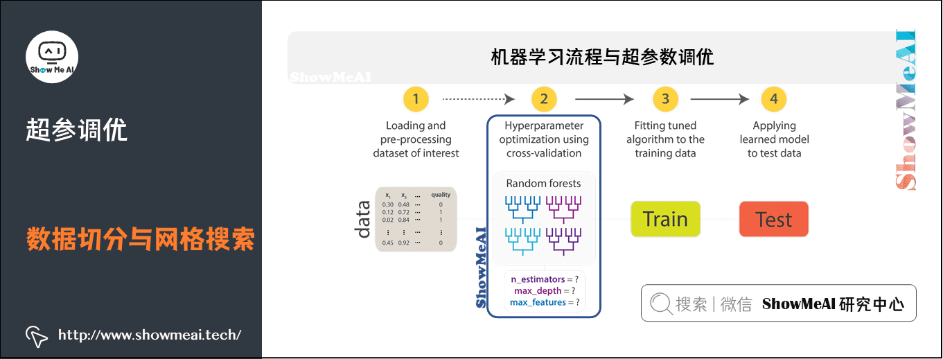
1) Machine learning process and super parameter optimization
In machine learning, model selection is a very important task.
- Using data to find the best model and parameters to solve specific problems is also called debugging
- Debugging can be done in an independent estimator (such as logistic regression) or in a workflow (including multiple algorithms, feature engineering, etc.)
- Users should tune the entire workflow at once, rather than individually tuning each component in the PipeLine
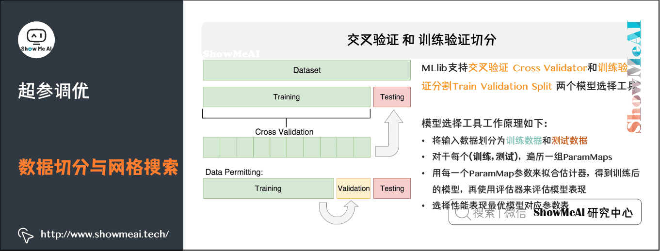
2) Cross validation and training validation segmentation
MLlib supports two model selection tools: Cross Validator and Train Validation Split. The requirements for using these tools include:
- Estimator: algorithm or pipeline to be debugged.
- The "parameters" table is also called "maps": a series of parameters.
- Evaluator: a criterion or method for evaluating the degree of fit of a model.
Cross validation CrossValidato divides the data set into k folded data sets, which are used for training and testing respectively. For example:
- When k=3, CrossValidator will generate 3 (training data and test data) pairs. The training data and test data of each data pair account for 2 / 3 and 1 / 3 respectively.
- In order to evaluate a ParamMap, CrossValidator will calculate the average evaluation index of the three different (training, testing) data sets on the model fitted by the Estimator.
- After finding the best ParamMap, CrossValidator will use this ParamMap and the entire dataset to re fit the Estimator.
In other words, find the best ParamMap through cross validation, and use this ParamMap to train (fit) an optimal model with strong generalization ability and relatively small error on the whole training set.
Cross validation is expensive. Therefore, Spark also provides training validation segmentation TrainValidationSplit for hyper parameter tuning.
- TrainValidationSplit creates a single (training, testing) dataset pair.
- It uses the trainRatio parameter to cut the dataset into two parts. For example, when trainRatio=0.75 is set, TrainValidationSplit will segment 75% of the data as the data set and 25% as the verification set to generate training and test set pairs, and finally use the best ParamMap and complete data set to fit the evaluator.
TrainValidationSplit only evaluates each parameter combination once, compared with k evaluations of each parameter by CrossValidator
- Therefore, the evaluation cost is low
- However, when the training data set is not large enough, the results are relatively unreliable
from pyspark.ml import Pipeline
from pyspark.ml.classification import LogisticRegression
from pyspark.ml.evaluation import BinaryClassificationEvaluator
from pyspark.ml.feature import HashingTF, Tokenizer
from pyspark.ml.tuning import CrossValidator, ParamGridBuilder
from pyspark.sql import SparkSession

spark = SparkSession\
    .builder\
    .appName("CrossValidatorExample")\
    .getOrCreate()

# $example on$
# Prepare training documents, which are labeled.
training = spark.createDataFrame([
    (0, "a b c d e spark", 1.0),
    (1, "b d", 0.0),
    (2, "spark f g h", 1.0),
    (3, "hadoop mapreduce", 0.0),
    (4, "b spark who", 1.0),
    (5, "g d a y", 0.0),
    (6, "spark fly", 1.0),
    (7, "was mapreduce", 0.0),
    (8, "e spark program", 1.0),
    (9, "a e c l", 0.0),
    (10, "spark compile", 1.0),
    (11, "hadoop software", 0.0)
], ["id", "text", "label"])

# Configure an ML pipeline, which consists of tree stages: tokenizer, hashingTF, and lr.
tokenizer = Tokenizer(inputCol="text", outputCol="words")
hashingTF = HashingTF(inputCol=tokenizer.getOutputCol(), outputCol="features")
lr = LogisticRegression(maxIter=10)
pipeline = Pipeline(stages=[tokenizer, hashingTF, lr])

# We now treat the Pipeline as an Estimator, wrapping it in a CrossValidator instance.
# This will allow us to jointly choose parameters for all Pipeline stages.
# A CrossValidator requires an Estimator, a set of Estimator ParamMaps, and an Evaluator.
# We use a ParamGridBuilder to construct a grid of parameters to search over.
# With 3 values for hashingTF.numFeatures and 2 values for lr.regParam,
# this grid will have 3 x 2 = 6 parameter settings for CrossValidator to choose from.
paramGrid = ParamGridBuilder() \
    .addGrid(hashingTF.numFeatures, [10, 100, 1000]) \
    .addGrid(lr.regParam, [0.1, 0.01]) \
    .build()

crossval = CrossValidator(estimator=pipeline,
                          estimatorParamMaps=paramGrid,
                          evaluator=BinaryClassificationEvaluator(),
                          numFolds=2)  # use 3+ folds in practice

# Run cross-validation, and choose the best set of parameters.
cvModel = crossval.fit(training)

# Prepare test documents, which are unlabeled.
test = spark.createDataFrame([
    (4, "spark i j k"),
    (5, "l m n"),
    (6, "mapreduce spark"),
    (7, "apache hadoop")
], ["id", "text"])

# Make predictions on test documents. cvModel uses the best model found (lrModel).
prediction = cvModel.transform(test)
selected = prediction.select("id", "text", "probability", "prediction")
for row in selected.collect():
    print(row)

spark.stop()
3. References
- Quick search of data science tools | Spark User Guide (RDD version) http://www.showmeai.tech/article-detail/106
- Quick search of data science tools | Spark User Guide (SQL version) http://www.showmeai.tech/article-detail/107
- Huang Meiling, Spark MLlib machine learning: detailed explanation of algorithm, source code and actual combat, electronic industry press, 2016
- Using ML Pipeline to build machine learning workflow https://www.ibm.com/developerworks/cn/opensource/os-cn-spark-practice5/index.html
- Spark official document: Machine Learning Library (MLlib) guide, http://spark.apachecn.org/docs/cn/2.2.0/ml-guide.html
ShowMeAI related articles recommended
- Illustrated big data | introduction: big data ecology and Application
- Graphic big data | distributed platform: detailed explanation of Hadoop and map reduce
- Illustrated big data | practical case: Hadoop system construction and environment configuration
- Illustrated big data | practical case: big data statistics using map reduce
- Illustrated big data | practical case: Hive construction and application case
- Graphic big data | massive database and query: detailed explanation of Hive and HBase
- Graphic big data | big data analysis and mining framework: Spark preliminary
- Graphic big data | Spark operation: big data processing analysis based on RDD
- Graphic big data | Spark operation: big data processing analysis based on Dataframe and SQL
- Illustrating big data covid-19: using spark to analyze the new US crown pneumonia epidemic data
- Illustrated big data | comprehensive case: mining retail transaction data using Spark analysis
- Illustrated big data | comprehensive case: Mining music album data using Spark analysis
- Graphic big data | streaming data processing: Spark Streaming
- Graphic big data | Spark machine learning (Part I) - workflow and Feature Engineering
- Graphical big data | Spark machine learning (Part 2) - Modeling and hyperparametric optimization
- Graphic big data | Spark GraphFrames: graph based data analysis and mining
ShowMeAI series tutorial recommendations
- Proficient in Python: Tutorial Series
- Graphic data analysis: a series of tutorials from introduction to mastery
- Fundamentals of graphic AI Mathematics: a series of tutorials from introduction to mastery
- Illustrated big data technology: a series of tutorials from introduction to mastery
- Graphical machine learning algorithms: a series of tutorials from introduction to mastery