Original link: http://tecdat.cn/?p=6663

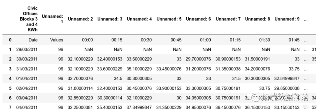
In this example, the neural network is used to predict the power consumption of citizens' offices using data from April 2011 to February 2013.

Daily data is created by totaling the consumption of 15 minute intervals provided each day.

Introduction to LSTM

LSTM (or short-term memory artificial neural network) allows the analysis of ordered data with long-term dependence. When it comes to this task, the traditional neural network shows deficiencies. In this regard, LSTM will be used to predict the power consumption mode in this case.

Compared with ARIMA and other models, a special advantage of LSTM is that the data does not necessarily need to be stable (constant mean, variance and autocorrelation) for LSTM to analyze it.

Autocorrelation diagram, Dickey fuller test and logarithmic transformation

To determine whether there is stationarity in our model:

• Generate autocorrelation and partial autocorrelation diagrams
• Conduct Dickey fuller test
• If any, change the above two time series to determine the stationarity (if any)

First, this is the time series diagram:

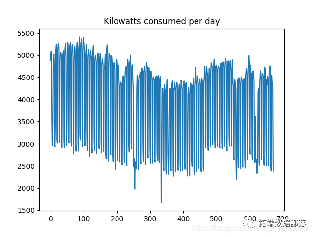
It is observed that volatility (or changes in consumption from one day to the next) is very high. In this regard, logarithmic transformation can be used to try to smooth the data slightly. Before that, ACF and PACF diagrams were generated and Dickey fuller test was performed.

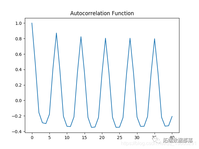
Autocorrelation diagram

Partial autocorrelation diagram

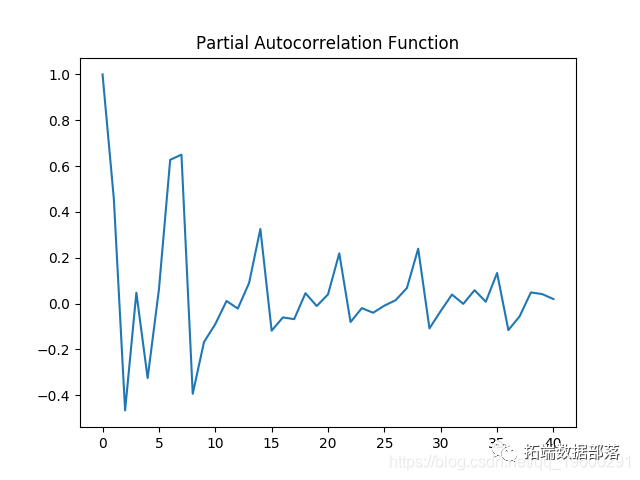
Both autocorrelation and partial autocorrelation plots show significant volatility, which means that several intervals in the time series have correlation.

When running the Dickey fuller test, the following results are produced:

When the p value is higher than 0.05, the null hypothesis of non stationarity cannot be rejected.

 STD1
954.7248
4043.4302
0.23611754

The coefficient of variation (or mean divided by standard deviation) is 0.236, indicating that the series has significant volatility.

The data is now converted to logarithmic format.

Although the time series is still unstable, when expressed in logarithmic format, the size of the deviation decreases slightly:

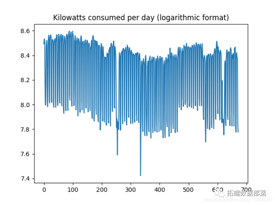
In addition, the coefficient of variation has decreased significantly to 0.0319, which means that the variability of the trend related to the average is significantly lower than that previously.

STD2 = np.std(Data set)
mean2 = np.mean(Data set)
cv2 = std2 / mean2 #Coefficient of variation

std2
 0.26462445

mean2
 8.272395

cv2
 0.031988855

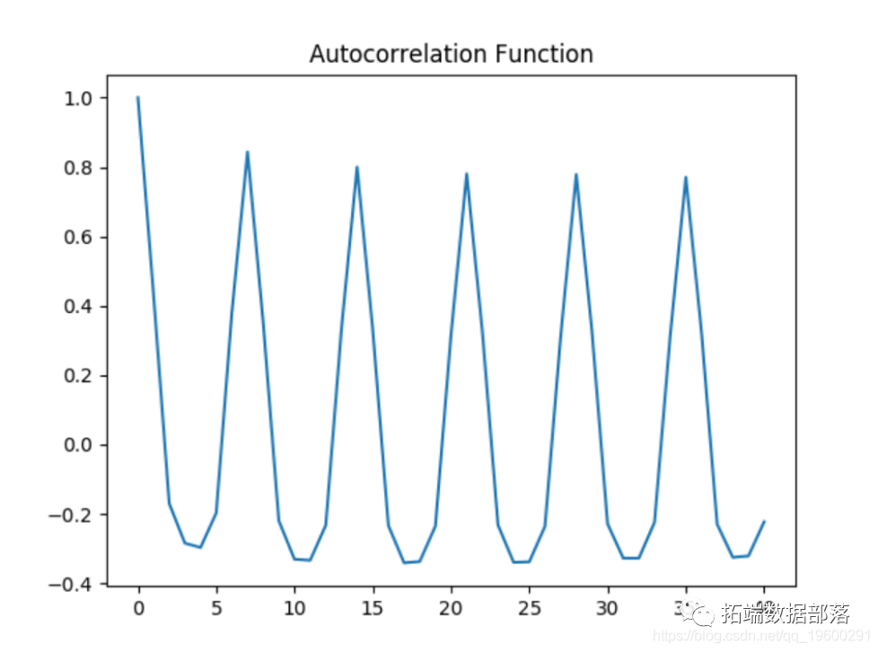
Similarly, ACF and PACF diagrams are generated on logarithmic data, and Dickey fuller test is performed again.

Autocorrelation diagram

Partial autocorrelation diagram

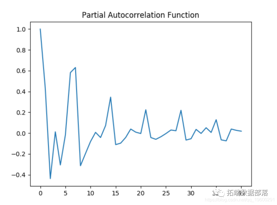
Dickey fuller test

... print('\ t％s: ％. 3f'％(key，value))
1％: -3.440
5％:  -  2.866
10％:  -  2.569

The p value of Dickey fuller test decreased to 0.0576. Although this does not technically reject the 5% significance threshold required for the null hypothesis, the logarithmic time series has shown lower volatility based on CV measurement, so the time series is used for the prediction purpose of LSTM.

Time series analysis of LSTM

Now, the LSTM model is used for prediction purposes.

data processing

First, import relevant libraries and perform data processing

LSTM generation and prediction

The model is trained for more than 100 periods and generates predictions.

＃generate LSTM network
model = Sequential()
model.add(LSTM(4，input_shape =(1，previous)))
 model.fit(X\_train，Y\_train，epochs = 100，batch_size = 1，verbose = 2)

＃Generate forecast
trainpred = model.predict(X_train)

＃Convert standardized data into original data
trainpred = scaler.inverse_transform(trainpred)

＃calculation RMSE
trainScore = math.sqrt(mean\_squared\_error(Y_train \[0\]，trainpred \[: ，0\]))
 
＃Training prediction
trainpredPlot = np.empty_like(dataset)
 
＃Test prediction

＃Draw all forecasts
inversetransform，= plt.plot(scaler.inverse_transform(dataset))

accuracy

The model shows that the root mean square error of the training data set is 0.24 and the root mean square error of the test data set is 0.23. The average kilowatt consumption (expressed in logarithmic format) is 8.27, which means that the error of 0.23 is less than 3% of the average consumption.

The following is the relationship between predicted consumption and actual consumption:

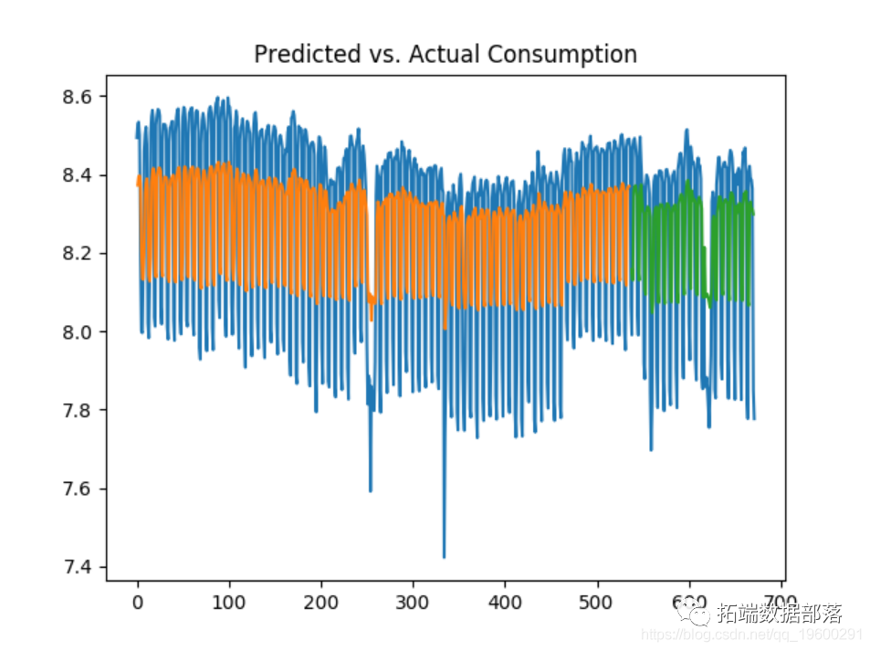
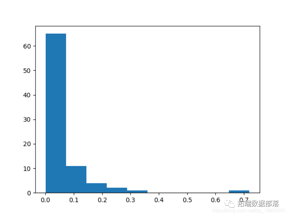
Interestingly, when the prediction is generated on the raw data (not converted to logarithmic format), the following training and test errors will occur:

When the average daily consumption is 4043 kW, the mean square error of the test accounts for nearly 20% of the total daily average consumption, and is very high compared with the error generated by logarithmic data.

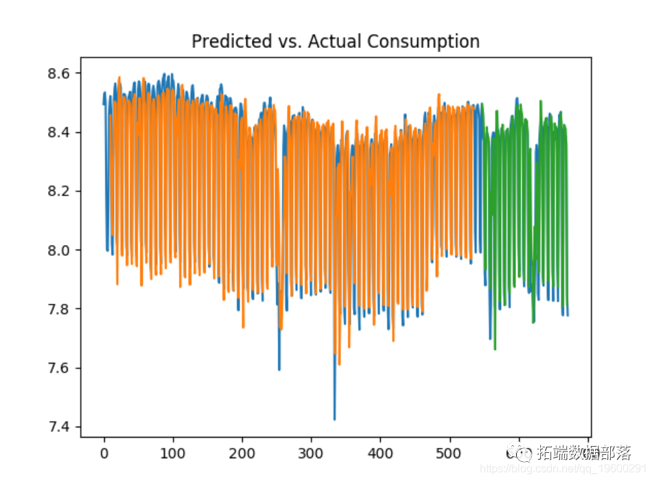
Let's look at this increase forecast to 10 and 50 days.

10 days

50 days

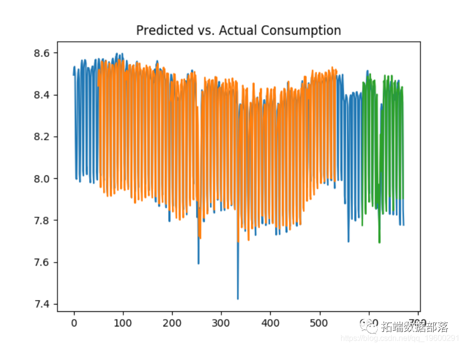
We can see that the test error decreases significantly between 10 and 50 days, and considering that the LSTM model considers more historical data in prediction, the volatility of consumption is better predicted.

Since the data is in logarithmic format, the predicted true value can now be obtained by obtaining the exponent of the data.

For example, the testred variable is readjusted with (1, - 1):

testpred.reshape(1，-1)
 array(\[\[7.7722197,8.277015,8.458941,8.455311,8.447589,8.445035，
 ......
8.425287,8.404881,8.457063,8.423954,7.98714,7.9003944，
8.240862,8.41654,8.423854,8.437414,8.397851,7.9047146\]\]，
dtype = float32)

conclusion

For this example, LSTM has proved to be very accurate in predicting power consumption fluctuations. In addition, the prediction accuracy of LSTM can be improved by representing the time series in logarithmic format.