Today is 815 tut7
Relevant contents of coursework part 2!!!

Let's start with the code
The first is the package introduced

# -*- coding: utf-8 -*-
"""
Created on Mon Mar  7 19:01:54 2022

@author: Pamplemousse
"""

#Set picture size
import matplotlib as mpl
mpl.rcParams['figure.figsize'] = [9.0, 6.0]

import nltk
from sklearn.datasets import load_files #Tools for reading files
from nltk.corpus import stopwords
import os
import string
from nltk.stem.porter import PorterStemmer
from nltk.stem.wordnet import WordNetLemmatizer
from sklearn.feature_extraction.text import CountVectorizer, TfidfTransformer, TfidfVectorizer
from sklearn.model_selection import train_test_split
from sklearn.linear_model import LogisticRegression #Logistic
from sklearn.discriminant_analysis import LinearDiscriminantAnalysis #Linear discriminator
from sklearn.naive_bayes import GaussianNB #Naive Bayes with Gaussian distribution a priori
from sklearn.svm import SVC #Support vector machine
from sklearn.metrics import classification_report, confusion_matrix, accuracy_score #Some goodness of fit tools
from sklearn.naive_bayes import MultinomialNB #Naive Bayes with a priori polynomial distribution
from sklearn.pipeline import Pipeline
import random
from functools import partial
from tabulate import tabulate
from yellowbrick.classifier import ClassificationReport
from yellowbrick.classifier import ConfusionMatrix
from sklearn.neural_network import MLPClassifier #artificial neural network

Setting of some parameters

default_stopwords = nltk.corpus.stopwords.words('english')#stopwords

lemma = WordNetLemmatizer()#lemmatize
porter_stemmer = PorterStemmer()#stemming

The text cleaning function is the same as last week's tut6 Part D & E. in fact, it can be copied directly, so there are no comments here

def clean_text(doc, rm_punctuation = True, rm_digits = True, lemmatize = False, 
               norm_case = True, stem = False, rm_stopwords = True):
    
    if(rm_punctuation == True):
        table = str.maketrans({key: None for key in string.punctuation})
        doc =str(doc).translate(table)
    
    if(rm_digits == True):
        table = str.maketrans({key: None for key in string.digits})
        doc = str(doc).translate(table)
    
    if(norm_case == True):
        doc = doc.lower()
    
    if(lemmatize == True):
        words = " ".join(lemma.lemmatize(word) for word in doc.split())
    else:
        words = " ".join([i for i in doc.split()])
    
    if(stem == True):
        words = " ".join(porter_stemmer.stem(word) for word in words.split())
    
    if(rm_stopwords == True):
        words = " ".join([i for i in words.split() if i not in default_stopwords])
    
    return words

The evaluation function of the model is then

def evaluate_model(model):
    
    model.fit(X_train, y_train)#Training model
    cr = ClassificationReport(model)#Classification report framework of model
    cr.score(X_test, y_test)#Test the model and get the data of the test results
    cr.finalize() #Here should be the action of drawing a thermal diagram of a report
    #In short, calling this function will get a thermodynamic diagram

read file

movie_dataDir = os.path.realpath("Desktop/King/815/Tutorial Week 7-20220307/Week6 Tutorial/txt_sentoken")
movie_data = load_files(movie_dataDir)
#load_files is a tool for reading text. Its return values include data, target and target_names

print(movie_data.target)

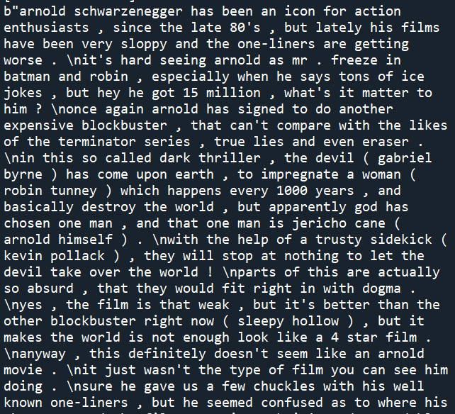
print(movie_data.data[0])

The output of the first print is
[0 1 1 ... 1 0 0]
P.S. the ellipsis in the middle is that the compiler cannot display so many, so it is omitted. It is not a real ellipsis
In movie_ data. The file type (0 / 1) is stored in target
The second print outputs the contents of the first file
Screenshot:

Then clean the text, that is, the movie_data.data processing

documents = [clean_text(x, stem = False, lemmatize = False) for x in movie_data.data]
#Call our custom clean_text() function

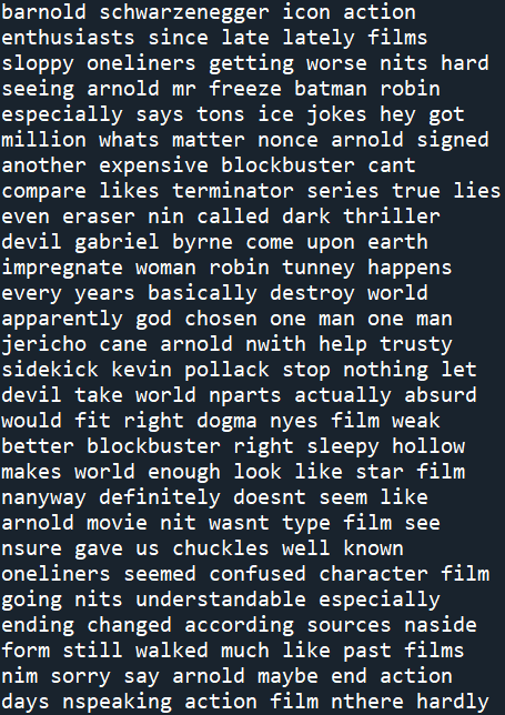
print(documents[0])#Output the first article to see the cleaning

Screenshot:

Then add document (argument) and movie_data.target (dependent variable) is converted into digit al data that can be processed by the computer

X,y = documents, movie_data.target

vectorizer = CountVectorizer(max_features = 1500, min_df = 5, max_df = 0.7, stop_words = stopwords.words('english'))#Word frequency converter
#After removing stopwords, the first 1500 words with a frequency of no more than 0.7 and a frequency of no less than 5
X = vectorizer.fit_transform(documents).toarray()#Construct word frequency vector

print(X[0][:10])#The first 10 data of word frequency vector in the first article

obtain
[0 0 0 0 0 0 0 0 0 5]
P.S. some words appear many times in the total, but the number of times in a single text may be 0. This word frequency vector represents the frequency of a word in the article

Then use the inverse text frequency index (idf) to convert the word frequency (tf). Please Baidu yourself

tfidfconverter = TfidfTransformer()
X = tfidfconverter.fit_transform(X).toarray()

print(X[0][:10])

The result is
[0. 0. 0. 0. 0. 0.
0. 0. 0. 0.24686232]

8: 2 separate training set and test set

X_train, X_test, y_train, y_test = train_test_split(X, y, test_size = 0.2, random_state = 0)

Then start running different classifiers and output the results
The first is logistic regression

logistic = LogisticRegression()
logistic.fit(X_train, y_train)

logistic_prediction = logistic.predict(X_test)

print(accuracy_score(logistic_prediction, y_test))
print(confusion_matrix(logistic_prediction, y_test))
print(classification_report(logistic_prediction, y_test))

accuracy score:
0.835

confusion matrix:
[[168 26]
[ 40 166]]

report:

	precision	recall	f1-score	support
0	0.81	0.87	0.84	194
1	0.86	0.81	0.83	106
accuracy			0.83	400
macro avg	0.84	0.84	0.83	400
weighted avg	0.84	0.83	0.83	400

P.S. I typed this form manually, but the result came out~

Linear discriminant model

lda = LinearDiscriminantAnalysis()
lda.fit(X_train, y_train)

lda_prediction = lda.predict(X_test)

print(accuracy_score(lda_prediction, y_test))
print(confusion_matrix(lda_prediction, y_test))
print(classification_report(lda_prediction, y_test))

accuracy score:
0.61

confusion matrix:
[[115 63]
[ 93 129]]

report:

	precision	recall	f1-score	support
0	0.55	0.65	0.60	178
1	0.67	0.58	0.62	222
accuracy			0.61	400
macro avg	0.61	0.61	0.61	400
weighted avg	0.62	0.61	0.61	400

Naive Bayes (Gaussian distribution)

nb = GaussianNB()
nb.fit(X_train, y_train)

nb_prediction = nb.predict(X_test)

print(accuracy_score(nb_prediction, y_test))
print(confusion_matrix(nb_prediction, y_test))
print(classification_report(nb_prediction, y_test))

accuracy score:
0.7625

confusion matrix:
[[164 51]
[ 44 141]]

report:

	precision	recall	f1-score	support
0	0.79	0.76	0.78	215
1	0.73	0.76	0.75	185
accuracy			0.76	400
macro avg	0.76	0.76	0.76	400
weighted avg	0.76	0.76	0.76	400

Support vector machine

SVC_model = SVC()
SVC_model.fit(X_train, y_train)

SVC_prediction = SVC_model.predict(X_test)

print(accuracy_score(SVC_prediction, y_test))
print(confusion_matrix(SVC_prediction, y_test))
print(classification_report(SVC_prediction, y_test))

accuracy score:
0.8275

confusion matrix:
[[167 28]
[ 41 164]]

report:

	precision	recall	f1-score	support
0	0.80	0.86	0.83	295
1	0.85	0.80	0.83	205
accuracy			0.83	400
macro avg	0.83	0.83	0.83	400
weighted avg	0.83	0.83	0.83	400

Then there is a large piece of pipeline, which is the pipeline
First build a pipeline model

model = Pipeline([
    ('tfidf', TfidfVectorizer()),
    ('clf', MultinomialNB()),
    ])#The model is first vectorized by tfidf, and then trained by naive Bayes (polynomial distribution)

model.fit(movie_data.data, movie_data.target)#Fitting model

Pipeline(steps=[('tfidf', TfidfVectorizer()), ('clf', MultinomialNB())])

Then we randomly select an article from the documents
Use the model to tfidf vectorize it, and then predict it

rantdoc = random.choice(documents)

print(rantdoc)

target = model.named_steps['tfidf'].transform([rantdoc])
target

print(model.predict([rantdoc]))

The output of rantdoc will not be posted here
Output of target:
<1x39659 sparse matrix of type '<class 'numpy.float64'>'
with 361 stored elements in Compressed Sparse Row format>

Predicted output:
[0]

But here we can't know whether the actual classification is 0 or 1, unless we compare the articles one by one

Output the probability of the prediction

tabulate = partial(tabulate, headers = 'firstrow', tablefmt = 'pipe')

probas = model.predict_proba([rantdoc])
table = [["Class", "Probability"]] + list(zip(model.classes_, probas[0]))
#Build probability table
print(tabulate(table))

Get this form

Class	Probability
0	0.689799
1	0.310201

P.S. when this output is copied to Markdown, it will naturally become a table. I like it
Therefore, for the prediction of this rantdoc, the probability of 0.6998 in this table is 0, so the previous output is 0

Then there is the visualization of the evaluation of model excellence, using the previous evaluate_model(), a custom function
Then we call this function for several classification models

evaluate_model(LogisticRegression())
evaluate_model(LinearDiscriminantAnalysis())
evaluate_model(GaussianNB())
evaluate_model(MultinomialNB())
evaluate_model(SVC())
evaluate_model(MLPClassifier())

P.S. the code here should be run line by line, otherwise there may be a problem with the output
The following thermodynamic diagram is obtained






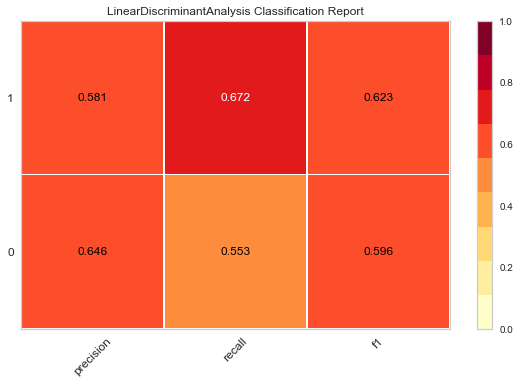
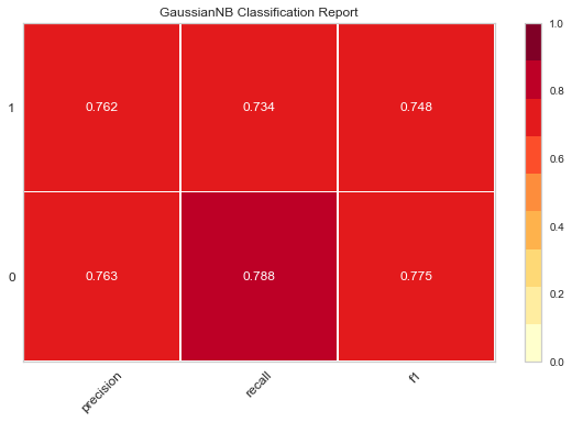
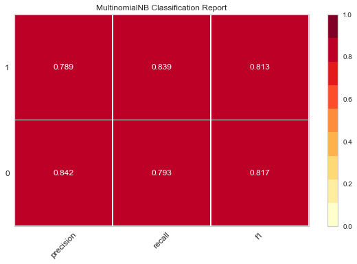
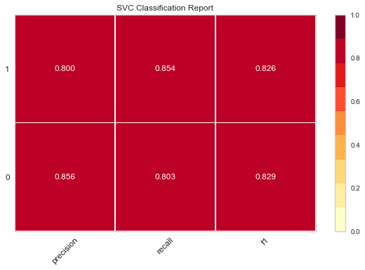
The darker the color of these thermal maps, the higher the value, and the better the effect

Then there is another way of visualization
Here, Logistic regression and linear discriminant analysis are operated. These two blocks should be run separately to get two results

viz = ConfusionMatrix(LogisticRegression())
viz.fit(X_train, y_train)
viz.score(X_test, y_test)
viz.poof()

viz = ConfusionMatrix(LinearDiscriminantAnalysis())
viz.fit(X_train, y_train)
viz.score(X_test, y_test)
viz.poof()

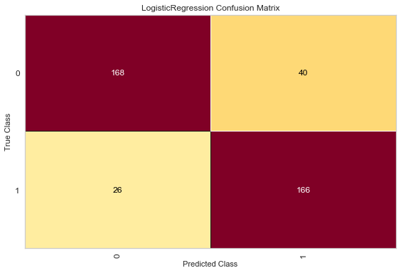
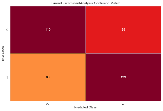
Here we want TP and TN to be larger, so the darker the upper left and lower right colors, the lighter the lower left and upper right colors, the better

Come on, everyone, coursework~
You can come to me if the security package is not good, you can also come to me if it is related to tutorial, you can also come to me if it is related to debug, and don't ask me if it is related to coursework
OK, get off work!