Recently, when arranging apprentice single-cell sharing, an apprentice mentioned GSE168522, which is a very standard six 10x single-cell transcriptome samples, as shown below:
GSM5145401 Sample 16_Normal-1
GSM5145402 Sample 17_Normal-2
GSM5145403 Sample 23_Early AD-1
GSM5145404 Sample 28_Early AD-2
GSM5145405 Sample 24_Late AD-1
GSM5145406 Sample 27_Late AD-2
However, the expression matrix provided by the author is not pure, but divided into different single-cell subsets:
GSE168522_B_cell_data.txt.gz 318.7 Kb
GSE168522_CD4_T_cell_data.txt.gz 317.3 Kb
GSE168522_CD8_T_cell_data.txt.gz 320.2 Kb
GSE168522_Gene_expression_of_six_samples_data.txt.gz 277.5 Kb
GSE168522_HSC_data.txt.gz 271.0 Kb
GSE168522_Monocytes_data.txt.gz 322.1 Kb
GSE168522_NK_cell_data.txt.gz 319.8 Kb
It's obvious that such a document can't give us a single-cell transcriptome process. Read the original: "single cell RNA sequencing requests B cell – related molecular biomarkers for Alzheimer's disease". In fact, it is introduced in single cell world: Single cell sequencing reveals B cell related markers of Alzheimer's disease
It can be seen that the number of cells in each 10x single-cell transcriptome sample mentioned in the original text is quite reasonable (5-8000), as shown below:
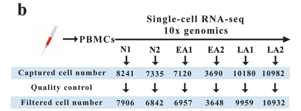
The number of cells is quite reasonable
The author's dimensionality reduction clustering is also super simple, which is just the first level. The immune cell subsets are subdivided, including two categories of lymphatic system (T,B,NK cells) and myeloid system (mononuclear, dendritic, macrophagy, granulocyte) as the second subdivision subsets:
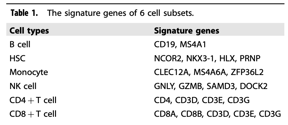
First level classification
Refer to the previous example: Single cell clustering and clustering annotation that everyone can learn It is also a simple look at the change of proportion:
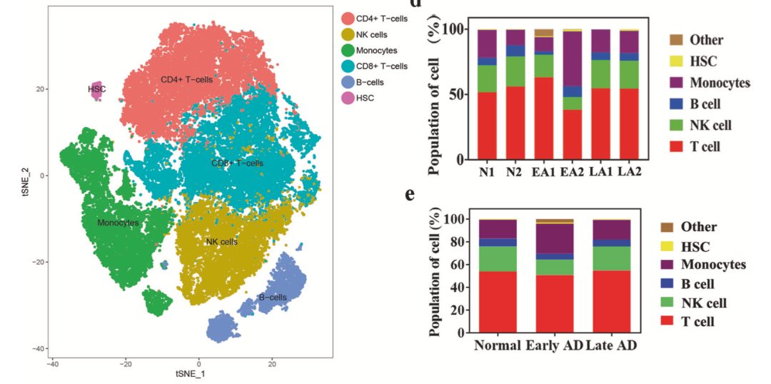
Proportional change
Since the author did not provide an expression matrix that can be analyzed directly, we need to start with the fastq sequencing data provided by him. Next, we will demonstrate this process:
Build Linux server operating environment
Install your own conda in the blank users of your server. Each user operates independently. The installation method code is as follows:
# First, download the file. It takes a few seconds for 20M/S
wget https://repo.anaconda.com/miniconda/Miniconda3-latest-Linux-x86_64.sh
# Next, use the bash command to run the file we downloaded. Remember to yes all the way
bash Miniconda3-latest-Linux-x86_64.sh
#  After successful installation, the system environment variable file needs to be updated
source ~/.bashrc
Next, use conda to install aspera. The code is as follows:
conda create -n download
conda activate download
conda install -y -c hcc aspera-cli
conda install -y -c bioconda sra-tools
which ascp
## Be sure to find out where your software is installed by conda
ls -lh ~/miniconda3/envs/download/etc/asperaweb_id_dsa.openssh
We have introduced the details of conda many times, so we won't repeat it here.
- conda management Shengxin software is enough
- Shengxin skill tree station B software installation video
- https://www.bilibili.com/video/av28836717
Next, configure the database file and software of cellranger:
Download the fastq file from the ENA database using aspera
First of all, you need the following address information. Go to the ENA database and follow the diagram to download it and build it into FQ Txt file:
fasp.sra.ebi.ac.uk:/vol1/fastq/SRR139/009/SRR13911909/SRR13911909_1.fastq.gz
fasp.sra.ebi.ac.uk:/vol1/fastq/SRR139/009/SRR13911909/SRR13911909_2.fastq.gz
fasp.sra.ebi.ac.uk:/vol1/fastq/SRR139/010/SRR13911910/SRR13911910_1.fastq.gz
fasp.sra.ebi.ac.uk:/vol1/fastq/SRR139/010/SRR13911910/SRR13911910_2.fastq.gz
fasp.sra.ebi.ac.uk:/vol1/fastq/SRR139/011/SRR13911911/SRR13911911_1.fastq.gz
fasp.sra.ebi.ac.uk:/vol1/fastq/SRR139/011/SRR13911911/SRR13911911_2.fastq.gz
fasp.sra.ebi.ac.uk:/vol1/fastq/SRR139/012/SRR13911912/SRR13911912_1.fastq.gz
fasp.sra.ebi.ac.uk:/vol1/fastq/SRR139/012/SRR13911912/SRR13911912_2.fastq.gz
fasp.sra.ebi.ac.uk:/vol1/fastq/SRR139/013/SRR13911913/SRR13911913_1.fastq.gz
fasp.sra.ebi.ac.uk:/vol1/fastq/SRR139/013/SRR13911913/SRR13911913_2.fastq.gz
fasp.sra.ebi.ac.uk:/vol1/fastq/SRR139/014/SRR13911914/SRR13911914_1.fastq.gz
fasp.sra.ebi.ac.uk:/vol1/fastq/SRR139/014/SRR13911914/SRR13911914_2.fastq.gz
Then write scripts and download them in batches;
cat fq.txt |while read id
do
ascp -QT -l 300m -P33001  \
-i ~/miniconda3/envs/download/etc/asperaweb_id_dsa.openssh   \
era-fasp@$id  .
done
This script will call aspera installed by conda to read FQ The paths in the txt file can be downloaded one by one, as shown below. From 8:30 p.m. to 1 a.m., all the fastq data files of our six 10x single cell transcriptome samples were downloaded successfully.
~$ ls -lh *gz|cut -d" " -f 5-
7.5G 1 September 29-20:25 SRR13911909_1.fastq.gz
 31G 1 September 29-20:53 SRR13911909_2.fastq.gz
7.5G 1 September 29-20:58 SRR13911910_1.fastq.gz
 31G 1 September 29-21:20 SRR13911910_2.fastq.gz
7.3G 1 September 29-21:28 SRR13911911_1.fastq.gz
 31G 1 September 29-21:53 SRR13911911_2.fastq.gz
7.2G 1 September 29-21:58 SRR13911912_1.fastq.gz
 30G 1 September 29-22:58 SRR13911912_2.fastq.gz
7.5G 1 September 29-23:15 SRR13911913_1.fastq.gz
 31G 1 June 30 00:12 SRR13911913_2.fastq.gz
7.2G 1 June 30 00:21 SRR13911914_1.fastq.gz
 30G 1 June 30 00:49 SRR13911914_2.fastq.gz
Run cellranger
At present, the single cell transcriptome is the mainstream of 10X company. We also introduced the details and processes of cellranger in detail in the single cell world official account.
- Single cell combat (I) data download
- Single cell combat (II) precautions before using cell ranger
- Single cell combat (III) preliminary study on the use of Cell Ranger
- Single cell combat (IV) overview of Cell Ranger process
- Single cell combat (V) understanding the results of cell Ranger count
However, this series of notes two years ago is based on V2 and V3 versions of cellranger. In July 2020, I saw that it was updated to V4, and a summary was also written in it. See: Cell Ranger updated to 4 (new tutorial)
The use method is super simple, that is to build a simple script. The code is as follows:
$ cat run-cellranger.sh
bin=/home/data/bylin/cellranger-6.1.2/bin/cellranger
db=/home/data/bylin/refdata-gex-GRCh38-2020-A
ls $bin; ls $db

fq_dir=/home/x9/raw
$bin count --id=$1 \
--localcores=4 \
--transcriptome=$db \
--fastqs=$fq_dir \
--sample=$1   \
--expect-cells=5000
The next step is to use this script to batch process our previous six 10x single cell transcriptome data.
The fastq file name starting with SRR in the front is modified uniformly:
Early_AD-1_S1_L001_R1_001.fastq.gz
Early_AD-1_S1_L001_R2_001.fastq.gz
Early_AD-2_S1_L001_R1_001.fastq.gz
Early_AD-2_S1_L001_R2_001.fastq.gz
Late_AD-1_S1_L001_R1_001.fastq.gz
Late_AD-1_S1_L001_R2_001.fastq.gz
Late_AD-2_S1_L001_R1_001.fastq.gz
Late_AD-2_S1_L001_R2_001.fastq.gz
Normal-1_Homo_S1_L001_R1_001.fastq.gz
Normal-1_Homo_S1_L001_R2_001.fastq.gz
Normal-2_Homo_S1_L001_R1_001.fastq.gz
Normal-2_Homo_S1_L001_R2_001.fastq.gz
You can see the file name of the comparison rule. Each sample is_ S1_L001_R1_001.fastq.gz and_ S1_ L001_ R2_ 001.fastq. At the end of GZ, the prefix in front is different for each sample, which is also the prefix used to distinguish different samples when we run the process later.
Therefore, you need to build a text file id.txt, which is as follows:
x9@bio1-2288H-V5:/home/data/x9$ cat id.txt
Early_AD-1
Early_AD-2
Late_AD-1
Late_AD-2
Normal-1_Homo
Normal-2_Homo
It has only six simple lines, which is the prefix of our fastq file.
A simple script can process all six 10x single cell transcriptome data files:
cat id.txt |while read id;do (nohup bash run-cellranger.sh $id 1>log-$id.txt 2>&1 & );done
You can see:
drwxrwxr-x 4 x9 x9 4.0K 1 February 30:55 Early_AD-1
drwxrwxr-x 4 x9 x9 4.0K 1 February 30:54 Early_AD-2
-rw-rw-r-- 1 x9 x9  140 1 September 29-20:41 id
-rw-rw-r-- 1 x9 x9   70 1 September 29-20:42 id.txt
drwxrwxr-x 4 x9 x9 4.0K 1 March 30:00 Late_AD-1
drwxrwxr-x 4 x9 x9 4.0K 1 February 30:51 Late_AD-2
-rw-rw-r-- 1 x9 x9  95K 1 February 30:55 log-Early_AD-1.txt
-rw-rw-r-- 1 x9 x9  96K 1 February 30:54 log-Early_AD-2.txt
-rw-rw-r-- 1 x9 x9  96K 1 March 30:00 log-Late_AD-1.txt
-rw-rw-r-- 1 x9 x9  95K 1 February 30:51 log-Late_AD-2.txt
-rw-rw-r-- 1 x9 x9  88K 1 February 30:44 log-Normal-1_Homo.txt
-rw-rw-r-- 1 x9 x9 9.6K 1 September 29-21:09 log-Normal-2_Homo.txt
drwxrwxr-x 4 x9 x9 4.0K 1 February 30:44 Normal-1_Homo
drwxrwxr-x 5 x9 x9 4.0K 1 September 29-21:09 Normal-2_Homo
Among them, 4.0K is the folder, 6 samples output 6 folders, and then 95K is the txt log. The log of each run of cellranger is kept and can be checked later. I'm running the command with x9 this user.
As you can see, it's basically a task that ends at 3 a.m. Next, you need to sort out the necessary contents in all successful folders. By default, multiple items are run under the same folder. You can see that the format in the folder corresponding to each sample is similar
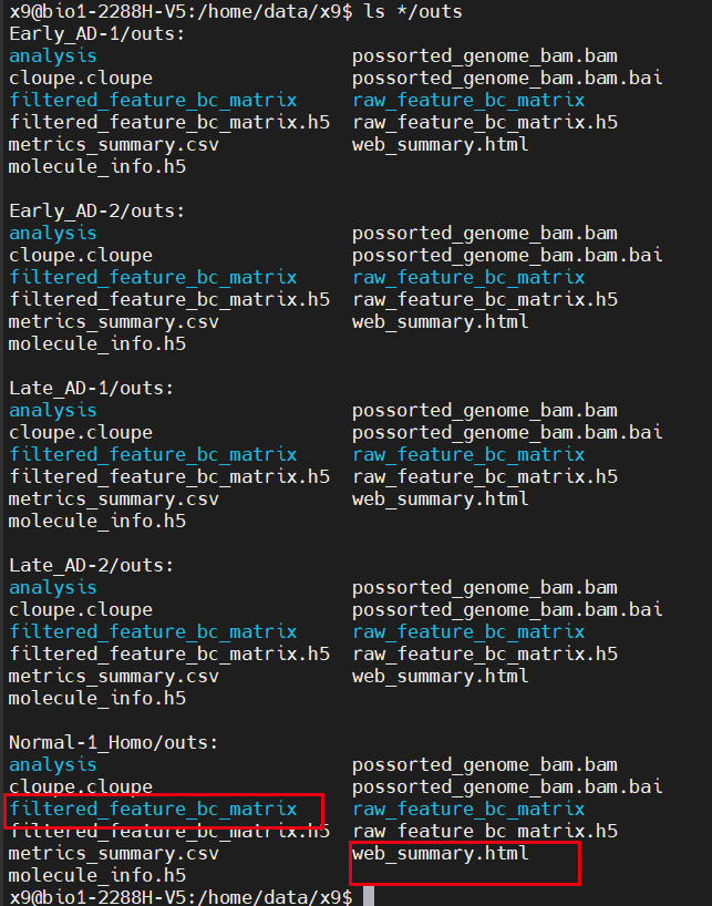
The format in the folder corresponding to each sample is similar
The most important one is filtered_ feature_ bc_ Contents in matrix folder and web_summary.html this report:
Still need to write a code:
pro=tmp
pro_folder=$HOME/$pro
mkdir -p $pro_folder
ls -lh  $pro_folder


mkdir -p $pro_folder/html
ls */outs/web_summary.html |while read id;do (cp $id $pro_folder/html/${id%%/*}.html );done

mkdir -p $pro_folder/matrix
ls -d */outs/filtered_feature_bc_matrix |while read id;do (cp -r  $id $pro_folder/matrix/${id%%/*} );done
In this way, our report and expression matrix are sorted out:
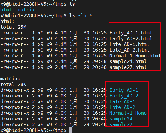
The report and expression matrix are sorted out
This is the end of the upstream process. The next step is to read the expression matrix of each sample and run the seurat process in R language. Each sample is an expression matrix composed of three files:
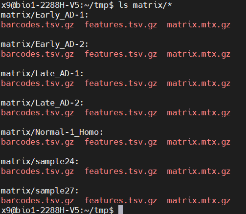
Each sample is an expression matrix composed of three documents
With such an expression matrix, it is easy to read it and follow the standard dimensionality reduction clustering process.
The first is to read six 10x single-cell transcriptome samples in batch
rm(list=ls())
options(stringsAsFactors = F)
library(Seurat)
library(ggplot2)
library(clustree)
library(cowplot)
library(dplyr)

###### step1:Import data ######
library(data.table)
dir='matrix/'
samples=list.files( dir )
samples

library(data.table)
sceList = lapply(samples,function(pro){
  # pro=samples[1]
  print(pro)
  sce=CreateSeuratObject( Read10X(file.path(dir,pro)),
                          project = pro,
                         min.cells = 5,
                         min.features = 300 )
  return(sce)
})
names(sceList)

samples
sce.all=merge(x=sceList[[1]],
              y=sceList[ -1 ],
              add.cell.ids = samples)

as.data.frame(sce.all@assays$RNA@counts[1:10, 1:2])
head(sce.all@meta.data, 10)
table(sce.all$orig.ident)
Then routine quality control and harmony integration are required:
sce = sce.all
sce <- NormalizeData(sce,
                         normalization.method = "LogNormalize",
                         scale.factor = 1e4)
sce <- FindVariableFeatures(sce)
sce <- ScaleData(sce)
sce <- RunPCA(sce, features = VariableFeatures(object = sce))

library(harmony)
seuratObj <- RunHarmony(sce, "orig.ident")
names(seuratObj@reductions)
seuratObj <- RunUMAP(seuratObj,  dims = 1:15,
                     reduction = "harmony")
DimPlot(seuratObj,reduction = "umap",label=T )

sce=seuratObj
sce <- FindNeighbors(sce, reduction = "harmony",
                     dims = 1:15)
sce.all=sce
#Set different resolutions and observe the clustering effect (which one to choose?)
for (res in c(0.01, 0.05, 0.1, 0.2, 0.3, 0.5,0.8,1)) {
  sce.all=FindClusters(sce.all, #graph.name = "CCA_snn",
                       resolution = res, algorithm = 1)
}
The next step is to visualize the marker gene we gave you and give it a reasonable name:
sce.all
sce=sce.all
library(ggplot2)
genes_to_check = c('PTPRC', 'CD3D', 'CD3E', 'CD4','CD8A',
                   'CD19', 'CD79A', 'MS4A1' ,
                   'IGHG1', 'MZB1', 'SDC1',
                   'CD68', 'CD163', 'CD14',
                   'TPSAB1' , 'TPSB2',  # mast cells,
                   'RCVRN','FPR1' , 'ITGAM' ,
                   'C1QA',  'C1QB',  # mac
                   'S100A9', 'S100A8', 'MMP19',# monocyte
                   'FCGR3A',
                   'LAMP3', 'IDO1','IDO2',## DC3
                   'CD1E','CD1C', # DC2
                   'KLRB1','NCR1', # NK
                   'FGF7','MME', 'ACTA2', ## fibo
                   'DCN', 'LUM',  'GSN' , ## mouse PDAC fibo
                   'MKI67' , 'TOP2A',
                   'PECAM1', 'VWF',  ## endo
                   'EPCAM' , 'KRT19', 'PROM1', 'ALDH1A1' )

library(stringr)
genes_to_check=str_to_upper(genes_to_check)
genes_to_check
p <- DotPlot(sce.all, features = unique(genes_to_check),
             assay='RNA'  )  + coord_flip()

p
ggsave('check_last_markers.pdf',height = 11,width = 11)
As follows:
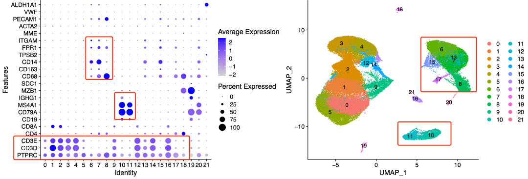
Dimension Reduction Clustering
It can be seen that immune cell subsets are subdivided, including two categories: lymphatic system (T,B,NK cells) and myeloid system (mononuclear, dendritic, macrophagy, granulocyte).
We give the name as follows:
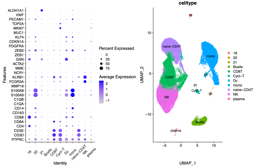
Biological nomenclature
Among them, I can't give the name for the first time on 18, 20 and 21. I need to follow up and explore slowly, but the results are consistent with the original text on the whole. What I didn't give a name may be that its marker genes are ncor2, NKX3-1, Hlx and PRNP, but they are not in the gene list I recited before.
However, knowledge is slowly increasing in this way!
If you really think my tutorial is helpful to your scientific research project and makes you enlightened, or your project uses a lot of my skills, please add a short thank you when publishing your achievements in the future, as shown below:
We thank Dr.Jianming Zeng(University of Macau), and all the members of his bioinformatics team, biotrainee, for generously sharing their experience and codes.
If I have traveled around the world in universities and research institutes (including Chinese mainland) in ten years, I will give priority to seeing you if you have such a friendship.