Reference link
Original address
https://github.com/paulQuei/a-star-algorithm?spm=a2c6h.12873639.0.0.21834662LgAvMP

A * algorithm for path planning

Algorithm Introduction

A * (read: A Star) algorithm is a very common path finding and graph traversal algorithm. It has better performance and accuracy. While explaining the algorithm, this paper will also provide the code implementation of Python language, and dynamically display the operation process of the algorithm with the help of matplotlib library.

A * algorithm was originally published in 1968 by Peter Hart, Nils Nilsson and Bertram Raphael of Stanford Research Institute. It can be considered as an extension of Dijkstra algorithm.

Due to the guidance of heuristic function, A * algorithm usually has better performance.

Breadth first search

In order to better understand the A * algorithm, let's start with the Breadth First algorithm.

As its name indicates, breadth first search takes breadth as its priority.

Starting from the starting point, first traverse the adjacent points around the starting point, and then traverse the adjacent points of the traversed points, and gradually spread outward until the end point is found.

This algorithm expands outward like Flood fill. The process of the algorithm is shown in the following figure:

In the above dynamic graph, the algorithm traverses all the points in the graph, which is usually unnecessary. For the problem with a clear end point, the algorithm can be terminated in advance once it reaches the end point. The following figure compares this situation:

In the process of executing the algorithm, each point needs to record the position of the previous point reaching the point - which can be called the parent node. After this, once you reach the end point, you can start from the end point, and then find the starting point in the order of the parent nodes, thus forming a path.

Dijkstra algorithm

Dijkstra algorithm was proposed by computer scientist Edsger W. Dijkstra in 1956.

Dijkstra algorithm is used to find the shortest path between nodes in the graph.

Considering such a scenario, in some cases, the moving costs between adjacent nodes in the graph are not equal. For example, if a picture in the game has both flat land and mountains, the speed of the characters in the game moving in the flat land and mountains is usually not equal.

In Dijkstra algorithm, the total moving cost of each node from the starting point needs to be calculated. At the same time, a priority queue structure is also needed. All nodes to be traversed are placed in the priority queue and sorted according to the cost.

In the process of running the algorithm, the node with the lowest cost is selected from the priority queue every time as the next traversal node. Until we reach the end.

The operation results of breadth first search without considering the difference of node mobility cost and Dijkstra algorithm considering mobility cost are compared below:

When the graph is a grid graph and the moving cost between each node is equal, the Dijkstra algorithm will become the same as the breadth first algorithm.

Best first search

In some cases, if we can calculate the distance from each node to the end point in advance, we can use this information to reach the end point faster.

The principle is also very simple. Similar to Dijkstra algorithm, we also use a priority queue, but at this time, the distance from each node to the end point is taken as the priority, and the node with the lowest moving cost to the end point (closest to the end point) is always selected as the next traversal node. This algorithm is called Best First algorithm.

This can greatly speed up the path search, as shown in the following figure:

But will this algorithm have any disadvantages? The answer is yes.

Because if there are obstacles between the start point and the end point, the best first algorithm may not find the shortest path. The following figure describes this situation.

A * algorithm

After comparing the above algorithms, we can finally explain the focus of this paper: A * algorithm.

In the following description, we will see that the A * algorithm actually integrates the characteristics of these algorithms.

A * algorithm calculates the priority of each node through the following function.

f ( n ) = g ( n ) + h ( n ) f(n) = g(n)+h(n) f(n)=g(n)+h(n)

Of which:

• f ( n ) f(n) f(n) is the comprehensive priority of node n. When we select the next node to traverse, we always select the node with the highest comprehensive priority (the lowest value).
• g ( n ) g(n) g(n) is the cost of node n from the starting point.
• h ( n ) h(n) h(n) is the estimated cost of node n from the end point, which is the heuristic function of A * algorithm. We will explain the heuristic function in detail below.

A * algorithm selects from the priority queue every time during operation f ( n ) f(n) The node with the lowest f(n) value (the highest priority) is the next node to be traversed.
In addition, the A * algorithm uses two sets to represent the nodes to be traversed and the nodes that have been traversed, which is usually called open_set and close_set.

The complete A * algorithm is described as follows:

* initialization open_set and close_set；
* Add starting point to open_set And set the priority to 0 (the highest priority);
* If open_set If it is not empty, the open_set Select the node with the highest priority n: 
    * If node n Is the end point, then:
        * Step by step tracking from the end point parent Node, reaching the starting point;
        * Return the found result path, and the algorithm ends;
    * If node n Not the end point, then:
        * Will node n from open_set Delete and join close_set Medium;
        * Traversal node n All adjacent nodes:
            * If adjacent nodes m stay close_set Medium, then:
                * Skip and select the next adjacent node
            * If adjacent nodes m Neither open_set Medium, then:
                * Set node m of parent As node n
                * Calculation node m Priority of
                * Will node m join open_set in

Heuristic function

As mentioned above, the heuristic function will affect the behavior of A * algorithm.

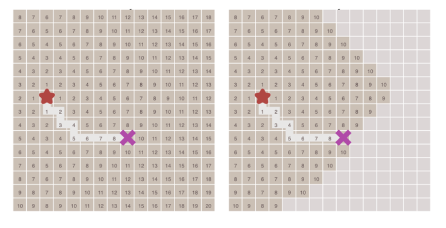
• In extreme cases, when the heuristic function h ( n ) h(n) If h(n) is always 0, then g ( n ) g(n) g(n) determines the priority of nodes, and the algorithm degenerates into Dijkstra algorithm.
• If h ( n ) h(n) If h(n) is always less than or equal to the cost of node n to the end point, the A * algorithm ensures that the shortest path can be found. But when h ( n ) h(n) The smaller the value of h(n), the more nodes the algorithm will traverse, and the slower the algorithm will be.
• If h ( n ) h(n) h(n) is exactly equal to the cost of node n to the end point, then the A * algorithm will find the best path, and the speed is very fast. Unfortunately, this is not possible in all scenarios. Because before we reach the end, it is difficult to calculate exactly how far we are from the end.
• If h ( n ) h(n) The value of h(n) is greater than the cost of node n to the end point, so the A * algorithm can not guarantee to find the shortest path, but it will be very fast at this time. At the other extreme, if h ( n ) h(n) h(n) relative to g ( n ) g(n) If g(n) is much larger, then only h ( n ) h(n) h(n) produces an effect, which becomes the best first search.

From the above information, we can know that we can control the speed and accuracy of the algorithm by adjusting the heuristic function. Because in some cases, we may not necessarily need the shortest path, but hope to find A path as soon as possible. This is also where the A * algorithm is more flexible.

For graphs in grid form, the following heuristic functions can be used:

• If you are only allowed to move up, down, left and right in the drawing, you can use Manhattan distance.
• If movement in eight directions is allowed in the drawing, you can use diagonal distances.
• If movement in any direction is allowed in the drawing, you can use Euclidean distance.

About distance

Manhattan distance

If only four directions are allowed to move up, down, left and right in the graph, the Manhattan distance can be used for the heuristic function, and its calculation method is shown in the following figure:

The function for calculating Manhattan distance is as follows. D here refers to the movement cost between two adjacent nodes, which is usually a fixed constant.

function heuristic(node) =
    dx = abs(node.x - goal.x)
    dy = abs(node.y - goal.y)
    return D * (dx + dy)

Diagonal distance

If oblique movement towards adjacent nodes is allowed in the graph, the heuristic function can use diagonal distance. Its calculation method is as follows:

The function for calculating the diagonal distance is as follows. D2 here refers to the moving cost between two adjacent nodes obliquely. If all nodes are square, the value is 2 ∗ D \sqrt{2} * D 2 ​∗D.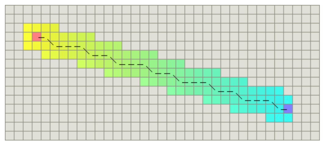

function heuristic(node) =
    dx = abs(node.x - goal.x)
    dy = abs(node.y - goal.y)
    return D * (dx + dy) + (D2 - 2 * D) * min(dx, dy)

Euclidean distance

If movement in any direction is allowed in the drawing, Euclidean distances can be used.

Euclidean distance refers to the straight-line distance between two nodes, so its calculation method is also familiar to us: ( p 2. x − p 1. x ) 2 + ( p 2. y − p 1. y ) 2 \sqrt{(p2.x-p1.x)^2 + (p2.y-p1.y)^2} (p2.x−p1.x)2+(p2.y−p1.y)2 ​. Its function is expressed as follows:

function heuristic(node) =
    dx = abs(node.x - goal.x)
    dy = abs(node.y - goal.y)
    return D * sqrt(dx * dx + dy * dy)

Algorithm implementation

The source code of the algorithm can be downloaded from github: Paul quei / a-star-algorithm.

Our algorithm demonstrates the solution process of finding the end point from the starting point on a two-dimensional grid graph.

Coordinate points and maps

First, we create a very simple class to describe the points in the diagram. The relevant codes are as follows:

# point.py

import sys

class Point:
    def __init__(self, x, y):
        self.x = x
        self.y = y
        self.cost = sys.maxsize

Next, we implement a class that describes the map structure. To simplify the description of the algorithm:

We select the point at the lower left coordinate [0, 0] as the starting point of the algorithm, and the point at the upper right coordinate [size - 1, size - 1] as the end point.

In order to make the algorithm more interesting, we set an obstacle in the middle of the map, and the map will also contain some random obstacles. The code of this class is as follows:

# random_map.py

import numpy as np

import point

class RandomMap:
    def __init__(self, size=50): # Constructor, the default size of the map is 50x50;
        self.size = size
        self.obstacle = size//8 # the number of obstacles is the map size divided by 8;
        self.GenerateObstacle() # Call generateobserver to generate random obstacles;

    def GenerateObstacle(self):
        self.obstacle_point = []
        self.obstacle_point.append(point.Point(self.size//2, self.size//2))
        self.obstacle_point.append(point.Point(self.size//2, self.size//2-1))

        # Generate an obstacle in the middle
        for i in range(self.size//2-4, self.size//2): # generate an oblique obstacle in the middle of the map;
            self.obstacle_point.append(point.Point(i, self.size-i))
            self.obstacle_point.append(point.Point(i, self.size-i-1))
            self.obstacle_point.append(point.Point(self.size-i, i))
            self.obstacle_point.append(point.Point(self.size-i, i-1))

        for i in range(self.obstacle-1):  # Several other obstacles are randomly generated;
            x = np.random.randint(0, self.size)
            y = np.random.randint(0, self.size)
            self.obstacle_point.append(point.Point(x, y))

            if (np.random.rand() > 0.5): # Random boolean the direction of obstacles is also random;
                for l in range(self.size//4):
                    self.obstacle_point.append(point.Point(x, y+l))
                    pass
            else:
                for l in range(self.size//4):
                    self.obstacle_point.append(point.Point(x+l, y))
                    pass

    def IsObstacle(self, i ,j): # Define a method to judge whether a node is an obstacle;
        for p in self.obstacle_point:
            if i==p.x and j==p.y:
                return True
        return False

Algorithm body

With the basic data structure, we can start to implement the algorithm body.

Here we use a class to encapsulate our algorithm.

First, implement some basic functions required by the algorithm, which are as follows:

# a_star.py

import sys
import time

import numpy as np

from matplotlib.patches import Rectangle

import point
import random_map

class AStar:
    def __init__(self, map): # __ init__:  Class.
        self.map=map
        self.open_set = []
        self.close_set = []

    def BaseCost(self, p): # Basepost: the moving cost from the node to the starting point, corresponding to g(n) above.
        x_dis = p.x
        y_dis = p.y
        # Distance to start point
        return x_dis + y_dis + (np.sqrt(2) - 2) * min(x_dis, y_dis)

    def HeuristicCost(self, p): # HeuristicCost: heuristic function from node to endpoint, corresponding to $h(n) $. Since we are a grid based graph, this function uses a diagonal distance from the previous function.
        x_dis = self.map.size - 1 - p.x
        y_dis = self.map.size - 1 - p.y
        # Distance to end point
        return x_dis + y_dis + (np.sqrt(2) - 2) * min(x_dis, y_dis)

    def TotalCost(self, p): # TotalCost: sum of costs, i.e. corresponding to f(n) mentioned above.
        return self.BaseCost(p) + self.HeuristicCost(p)

    def IsValidPoint(self, x, y): # IsValidPoint: judge whether the point is valid. It is invalid if it is not inside the map or where the obstacle is located.
        if x < 0 or y < 0:
            return False
        if x >= self.map.size or y >= self.map.size:
            return False
        return not self.map.IsObstacle(x, y)

    def IsInPointList(self, p, point_list): # Determine whether the point is in a set.
        for point in point_list:
            if point.x == p.x and point.y == p.y:
                return True
        return False

    def IsInOpenList(self, p): # Judge whether the point is open_set.
        return self.IsInPointList(p, self.open_set)

    def IsInCloseList(self, p): # Judge whether the point is closed_ Set.
        return self.IsInPointList(p, self.close_set)

    def IsStartPoint(self, p): # Judge whether the point is the starting point.
        return p.x == 0 and p.y ==0

    def IsEndPoint(self, p): # Judge whether the point is the end point.
        return p.x == self.map.size-1 and p.y == self.map.size-1

With the above auxiliary functions, you can start to implement the main logic of the algorithm. The relevant codes are as follows:

# a_star.py
def RunAndSaveImage(self, ax, plt):
    start_time = time.time()

    start_point = point.Point(0, 0)
    start_point.cost = 0
    self.open_set.append(start_point)

    while True:
        index = self.SelectPointInOpenList()
        if index < 0:
            print('No path found, algorithm failed!!!')
            return
        p = self.open_set[index]
        rec = Rectangle((p.x, p.y), 1, 1, color='c')
        ax.add_patch(rec)
        self.SaveImage(plt)

        if self.IsEndPoint(p):
            return self.BuildPath(p, ax, plt, start_time)

        del self.open_set[index]
        self.close_set.append(p)

        # Process all neighbors
        x = p.x
        y = p.y
        self.ProcessPoint(x-1, y+1, p)
        self.ProcessPoint(x-1, y, p)
        self.ProcessPoint(x-1, y-1, p)
        self.ProcessPoint(x, y-1, p)
        self.ProcessPoint(x+1, y-1, p)
        self.ProcessPoint(x+1, y, p)
        self.ProcessPoint(x+1, y+1, p)
        self.ProcessPoint(x, y+1, p)

This code should not need much explanation. It is implemented according to the previous algorithm logic. In order to show the results, we will save the state into pictures with the help of matplotlib library at each step of the algorithm.

The above function calls several other functions, and the code is as follows:

# a_star.py
def SaveImage(self, plt):
    millis = int(round(time.time() * 1000))
    filename = './' + str(millis) + '.png'
    plt.savefig(filename)

def ProcessPoint(self, x, y, parent):
    if not self.IsValidPoint(x, y):
        return # Do nothing for invalid point
    p = point.Point(x, y)
    if self.IsInCloseList(p):
        return # Do nothing for visited point
    print('Process Point [', p.x, ',', p.y, ']', ', cost: ', p.cost)
    if not self.IsInOpenList(p):
        p.parent = parent
        p.cost = self.TotalCost(p)
        self.open_set.append(p)

def SelectPointInOpenList(self):
    index = 0
    selected_index = -1
    min_cost = sys.maxsize
    for p in self.open_set:
        cost = self.TotalCost(p)
        if cost < min_cost:
            min_cost = cost
            selected_index = index
        index += 1
    return selected_index

def BuildPath(self, p, ax, plt, start_time):
    path = []
    while True:
        path.insert(0, p) # Insert first
        if self.IsStartPoint(p):
            break
        else:
            p = p.parent
    for p in path:
        rec = Rectangle((p.x, p.y), 1, 1, color='g')
        ax.add_patch(rec)
        plt.draw()
        self.SaveImage(plt)
    end_time = time.time()
    print('===== Algorithm finish in', int(end_time-start_time), ' seconds')

These three functions should be easy to understand:

• SaveImage: saves the current state to a picture named after the current time.
• ProcessPoint: process each node: if it is a node that has not been processed, calculate the priority, set the parent node, and add it to open_set.
• SelectPointInOpenList: from open_ Find the node with the highest priority in set and return its index.
• BuildPath: construct the result path from the end point back along the parent. Then draw the result from the starting point. The result uses a green square. Each drawing step saves one picture.

Test entrance

Finally, the entry logic of the program. Use the class written above to find the path:

# main.py

import numpy as np
import matplotlib.pyplot as plt

from matplotlib.patches import Rectangle

import random_map
import a_star

plt.figure(figsize=(5, 5))

map = random_map.RandomMap() ①

ax = plt.gca()
ax.set_xlim([0, map.size]) ②
ax.set_ylim([0, map.size])

for i in range(map.size): ③
    for j in range(map.size):
        if map.IsObstacle(i,j):
            rec = Rectangle((i, j), width=1, height=1, color='gray')
            ax.add_patch(rec)
        else:
            rec = Rectangle((i, j), width=1, height=1, edgecolor='gray', facecolor='w')
            ax.add_patch(rec)

rec = Rectangle((0, 0), width = 1, height = 1, facecolor='b')
ax.add_patch(rec) ④

rec = Rectangle((map.size-1, map.size-1), width = 1, height = 1, facecolor='r')
ax.add_patch(rec) ⑤

plt.axis('equal') ⑥
plt.axis('off')
plt.tight_layout()
#plt.show()

a_star = a_star.AStar(map)
a_star.RunAndSaveImage(ax, plt) ⑦

This code is described as follows:

1. Create a random map;
2. Set the content of the image to be consistent with the map size;
3. Draw a map: draw a gray square for obstacles and a white square for other areas;
4. The drawing starting point is a blue square;
5. The drawing end point is a red square;
6. Set the coordinate axis scale of the image to be equal and hide the coordinate axis;
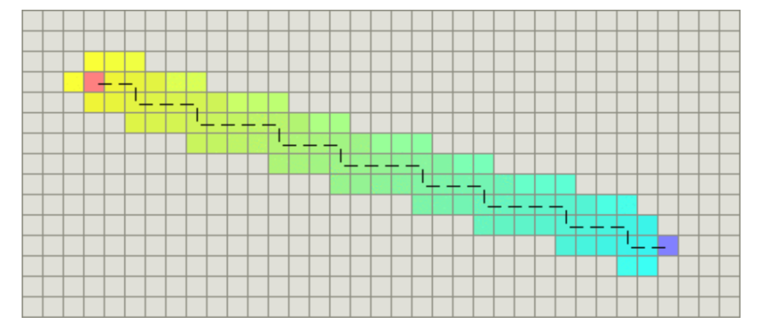
7. Call the algorithm to find the path;

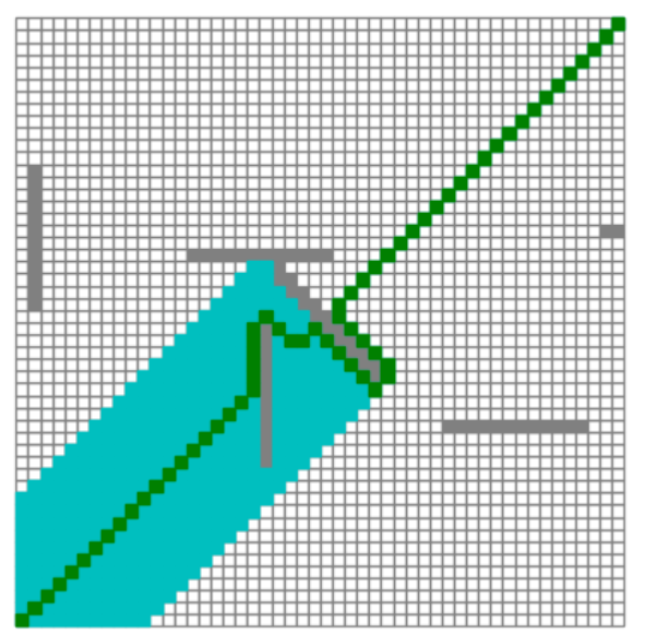
Since our map is random, the results of each run may be different. Here are the results of a run on my computer: