preface
We are students of domestic colleges and universities and beginners of quantitative investment. Our school is not reopened in northern Qing Dynasty, nor does it have a financial engineering laboratory. At the same time, it is located in a third tier town. Therefore, it is difficult for us to obtain quantitative internship opportunities during our school period, but we look forward to communicating and communicating with the industry.
Cai Jinhang is one of us. When looking for the quantitative internship in summer, he received the written examination invitation from several private placement and brokerage metalworking groups. The written examination content is to reproduce a metalworking Research Report within a given time. Inspired, Cai found that reproducing the metalworking research report is not only a good way for us to learn quantitative strategies, exercise program design ability, but also a good way to communicate with the industry.
At the suggestion of CAI, we started the creation of the reproduction series of the research report, recorded our learning process, shared our creative content, and communicated, studied and made progress with readers.
Our level is limited, and the content of our creation will inevitably have errors or imprecise content. We welcome readers' criticism and correction.
If you are interested in our content, please contact us: cai_jinhang@foxmail.com
Author:
Cai Jinhang, School of computer science and technology, Weihai campus, Harbin Institute of Technology
Shu Yiming, School of automotive engineering, Weihai campus, Harbin Institute of Technology
1. General
This is the fifth article of our research report. This article reproduces the [volume is just when entering the market: a preliminary study on the timing of trading volume] of Everbright Securities. The main idea of this research report is to enter the market at the time of trading volume based on the theory of "value first". The traditional way of describing trading volume is that the trading volume increases continuously for several days, but this situation is relatively rare in the market. This research report uses the relative ranking position between the trading volume of this day and the trading volume of the previous N days, maps it to the interval of [- 1,1], names this factor as the trading volume time series ranking factor, and uses this factor to quantify the volume degree of trading volume.
Build a variety of strategies based on the trading volume time series ranking factor.
The original trading volume time series ranking strategy is to select a opening and closing position threshold. The factor is greater than the threshold and less than the threshold.
After that, with the help of price optimization, the market is divided into bear market, bull market and shock market through price increase. Different market prices adopt different opening and closing thresholds. This strategy is called trading volume time series ranking market segmentation strategy.
Finally, the market segmentation strategy is combined with RSRS strategy, and the signals of the two strategies are processed differently in different markets.
This research paper reproduces and shares part of the source code of our research process.
2. Research environment
Python3
Data source: youkuang
Back test interval: March 2005 to may 2021
import pandas as pd
import matplotlib.pyplot as plt
from matplotlib.font_manager import FontProperties
import matplotlib as mpl
import datetime
import numpy as np
import statsmodels.api as sm
import math
import warnings
import seaborn as sns
sns.set()
warnings.filterwarnings('ignore')
plt.rcParams['font.sans-serif']=['SimHei']
plt.rcParams['axes.unicode_minus'] = False
Data acquisition function, whose function is to obtain data and change the field name.
def get_data(security,start_date,end_date):
    df = DataAPI.MktIdxdGet(
        ticker=security,
        beginDate=start_date,
        endDate=end_date,
        field=["tradeDate","openIndex","closeIndex","highestIndex","lowestIndex","turnoverVol"],
        pandas="1"
    )
    df = df.rename({
        'tradeDate':'datetime',
        'openIndex':'open',
        'closeIndex':'close',
        'highestIndex':'high',
        'lowestIndex':'low',
        'turnoverVol':'volume'
    },axis=1)
    df['ma20'] = pd.Series.rolling(df['close'],window = 20).mean()
    return df
3. Index construction and analysis
3.1 construction method of trading volume time series ranking index:
1. In addition to the trading volume of the day, we also need to take the daily trading volume of the previous N trading days
Trading volume data, a total of N+1 trading volume values.
2. Sort the N+1 trading volume data from small to large, and calculate the trading volume of the day here
Rank n among N+1 values, the smallest is 1, and the largest is N+1.
3. Standardize the daily trading volume ranking into the number within [- 1,1] through the operation (2 * n-n-2) / n
Value.
It should be noted here that the formula of the third point was given 2 * (n-N-1) / N in the original research report, which is wrong and cannot standardize the ranking to [- 1,1]
The function for calculating the factor is as follows:
def calc_rank_factor(df,N):
    df = df.copy()
    rank_list = [np.nan]*N
    for i in range(N,df.shape[0]):
        sorted_vol = list(df['volume'][i-N:i+1])
        sorted_vol = sorted(sorted_vol)
        rank_list.append(sorted_vol.index(df['volume'][i])+1)#Get ranking
    df['rank'] = rank_list
    df['rank_factor'] = (2*df['rank'] - N -2)/N#Standardization
    return df
3.2 factor analysis
Taking N=40 as an example, the trading volume time series ranking factor is calculated on CSI 300, and the characteristics of the factor are analyzed.
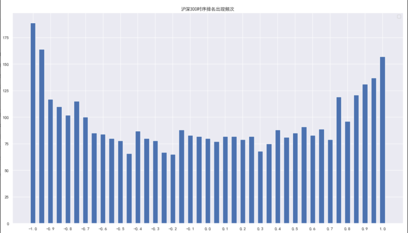
3.2.1 occurrence frequency of time series ranking
rank_factor_count = df['rank_factor'].value_counts()
rank_factor_count = dict(rank_factor_count)
plt.figure(figsize=(18,10))
plt.bar(rank_factor_count.keys(),rank_factor_count.values(), align='center',width=0.03)
plt.xticks(sorted(list(rank_factor_count.keys()))[::2],sorted(list(rank_factor_count.keys()))[::2])
fig_style(plt,title=f'Frequency of CSI 300 time series ranking')
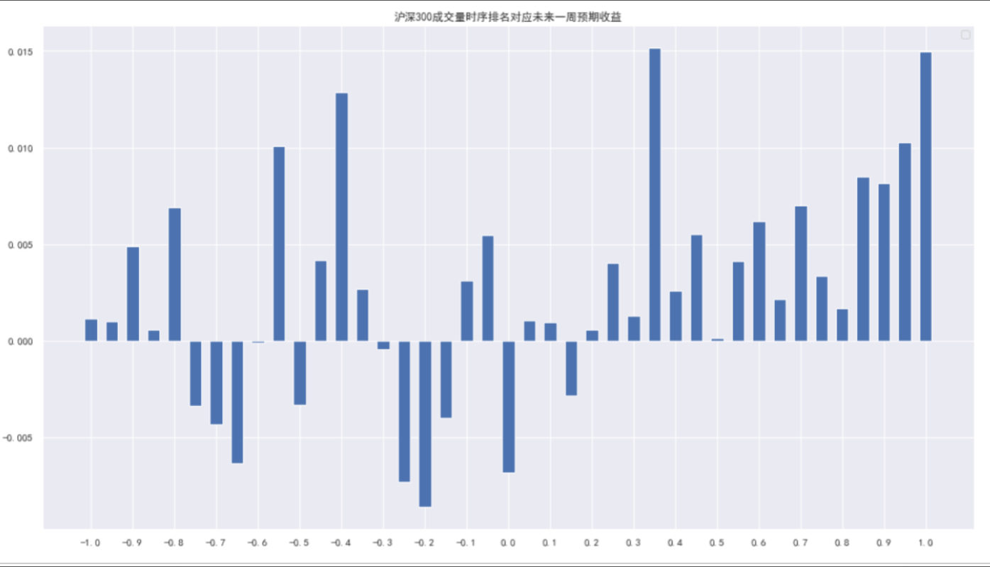
3.2.2 time series ranking factor and expected rate of return in the next week
df['week_ret'] = (df['close'].shift(-5) - df['close'])/df['close']
avg_week_ret_dic = {}
week_ret_by_factor = df.groupby(by='rank_factor')
for factor,df1 in week_ret_by_factor:
    avg_week_ret_dic
    [factor] = df1['week_ret'].mean()
avg_week_ret = pd.DataFrame({
    'rank_factor':list(avg_week_ret_dic.keys()),
    'week_ret':list(avg_week_ret_dic.values())
}).sort_values(by='rank_factor').reset_index(drop=True)
plt.figure(figsize=(18,10))
plt.bar(avg_week_ret['rank_factor'],avg_week_ret['week_ret'], align='center',width=0.03)
plt.xticks(avg_week_ret['rank_factor'][::2],avg_week_ret['rank_factor'][::2])
fig_style(plt,title=f'The time series ranking of trading volume of CSI 300 corresponds to the expected return in the next week')
4 strategy construction
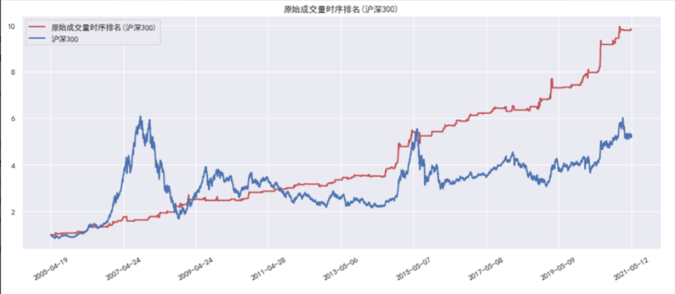
4.1 time series ranking strategy of original trading volume
We construct the timing strategy according to the time series ranking of single day trading volume. The specific methods are as follows:
1. Calculate the trading volume time series ranking of the current day index and standardize it into the index value in the [- 1,1] value range.
(involving parameter selection N, timing ranking window length)
2. When the trading volume time series ranking is within the maximum range, or equivalent, it will be standardized
The value of exceeds a certain threshold S (for example, the timing ranking is in the top quarter of the largest, or
If the standardized value exceeds 0.5), open the position and buy. (involving parameter selection S,
Opening threshold)
3. When the trading volume time series ranking leaves the high position, or equivalent, its standardized value is lower than a certain value
Threshold S, then close the position and wait and see.
4. No short selling and short selling.
The policy code is as follows:
def run_original_strategy(df,N,S):
    df = df.copy()
    df = df.copy()
    df = calc_rank_factor(df,N)
    df['flag'] = 0
    df['position'] = 0
    position = 0
    df = df.dropna().reset_index(drop=True)
    for i in range(df.shape[0]):
        if df.loc[i,'rank_factor']>S and position == 0:
            df.loc[i,'flag']=1
            df.loc[i+1,'position'] = 1
            position = 1
        elif df.loc[i,'rank_factor']<S and position == 1:
            df.loc[i,'flag']=-1
            df.loc[i+1,'position'] = 0
            position = 0
        else:
            df['position'][i+1] = df['position'][i]
    return df.dropna()
The net value trend of the strategy is shown in the figure below
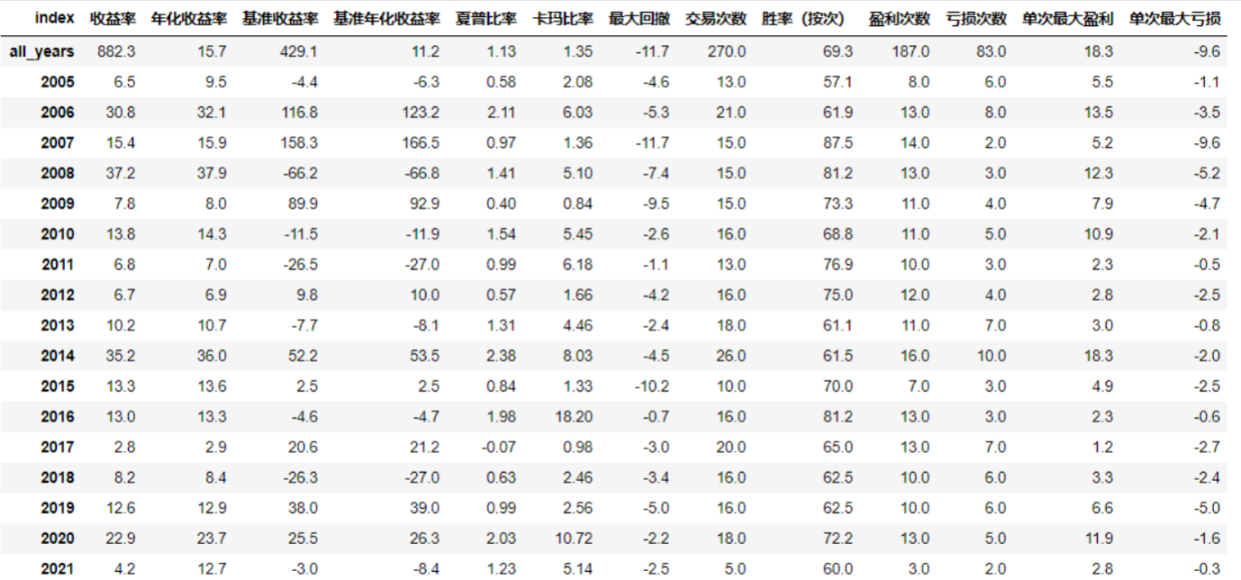
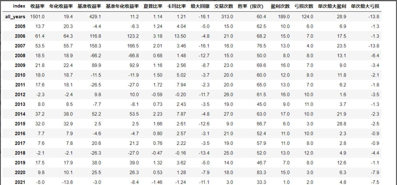
The statistical indicators of the strategy are shown in the figure below
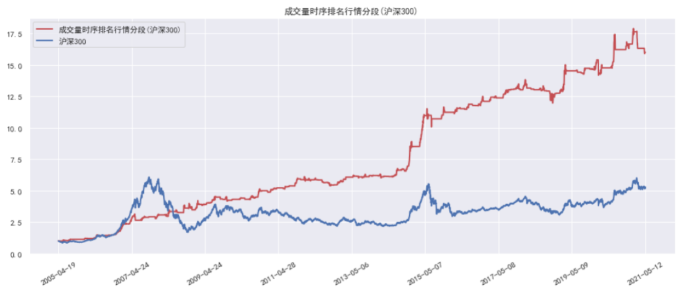
4.2 trading volume time series ranking and market segmentation strategy
In different market environments, the interpretation of trading volume information may also change. From the perspective of predicting the future market trend, when the market is in a bull market, the trading volume may be slightly large, or even as long as it does not shrink, it indicates that the future market probability will continue to rise; In a bear market, it may only rebound in the future when the trading volume is large. We segment the market through the increase of the index in the first 10 days, and study the predictive effect of the trading volume timing ranking on the future index trend under different market conditions. If the index rose less than - 5% in the first 10 days, it is considered to be in a bear market; If the index rose more than 5% in the first 10 days, it is considered to be in a bull market; If the index rose between - 5% and 5% in the first 10 days, it is considered to be a volatile market.
Therefore, the trading volume time series ranking market segmentation strategy is constructed in the following way:
- Calculate the standardized trading volume time series ranking index value of the day according to the definition of the previous chapter.
- According to the index increase of the previous 10 days, decide which market situation you are in that day: bull market, bear market, or shock market. Threshold for market division (default: 5%)
- According to the market situation of the day, different trading thresholds are used to determine the position of tomorrow. (parameters involved: Trading thresholds Sf, Sc and Sr under three different markets, corresponding to bear market, shock market and bull market respectively)
- If the time series ranking index value is greater than the transaction threshold, the position will be held; Otherwise, it will be empty.
Policy code:
def divide_market(df,C):
    df['10days_ret'] = df['close'].pct_change(10)
    df['market'] = ''
    df['market'].iloc[df[df['10days_ret']>C].index] = 'r'
    df['market'].iloc[df[(df['10days_ret']<=C)&(df['10days_ret']>=-1*C)].index] = 'c'
    df['market'].iloc[df[(df['10days_ret']<-1*C)].index] = 'f'
    return df

def run_market_strategy(df,N,C,Sf,Sc,Sr):
    df = df.copy()
    df = calc_rank_factor(df,N)
    df = divide_market(df,C)
    S_dict = {'f':Sf,'c':Sc,'r':Sr}
    df['flag'] = 0
    df['position'] = 0
    position = 0
    df = df.replace('',np.nan)
    df = df.dropna().reset_index(drop=True)
    for i in df.index:
        if df['rank_factor'][i]>S_dict[df['market'][i]] and position == 0:
            df['flag'][i]=1
            df['position'][i+1] = 1
            position = 1
        elif df['rank_factor'][i]<S_dict[df['market'][i]] and position == 1:
            df['flag'][i]=-1
            df['position'][i+1] = 0
            position = 0
        else:
            df['position'][i+1] = df['position'][i]
    return df.dropna()
The performance of the strategy is shown in the figure below
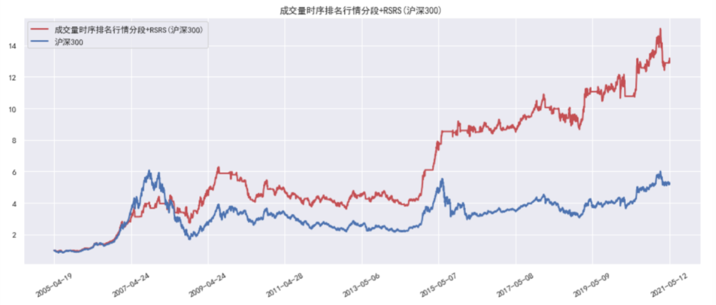
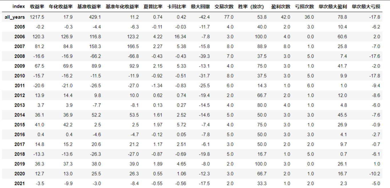
4.3 trading volume time series ranking market segmentation strategy + RSRS
Finally, we further try to combine the time series ranking index of market segmented trading volume with the RSRS timing signal constructed by the highest price and lowest price data. The reason and purpose of our doing this is: through the combination of signals, the defect that the trading volume timing ranking has too little time to hold positions in the bull market can be further compensated by the RSRS timing strategy, and at the same time, its ability to capture the long-term rebound opportunity in the volatile market and bear market can be retained as much as possible.
The combination method is as follows:
1. Obtain the signals of the time sequence ranking strategy and RSRS timing strategy of the market segment trading volume of the current day.
2. Follow the market segmentation method in the previous section to determine the market situation of the day: bull market, shock market or bear market.
3. Decide the timing signal according to the market of the day:
a) If the market is a bull market, it is completely based on the RSRS signal as the timing signal.
b) If the market is a volatile market, any strategy will hold a position when it gives a long signal, and will only be short when all signals are cautious. (or relationship)
c) If the market is a bear market, you must look at all the signals for a long time before you hold a position, otherwise you are short. (relationship with)
Policy code:
def calc_nbeta(df,n=18):
    nbeta = []
    r2 = []
    trade_days = len(df.index)
    for i in range(trade_days):
        if i < (n-1):
            #In order to match n-1, the iloc index is used next
            nbeta.append(np.nan)
            r2.append(np.nan)
        else:
            try:
                x = df['low'].iloc[i-n+1:i+1]
                #iloc left closed right open
                x = sm.add_constant(x)
                y = df['high'].iloc[i-n+1:i+1]
                regr = sm.OLS(y,x)
            except:
                print(x,y)
            res = regr.fit()
            beta = round(res.params[1],2)
            nbeta.append(beta)
            r2.append(res.rsquared)
    df1 = df.copy()
    df1 = df1.reset_index(drop=True)
    df1['beta'] = nbeta
    df1['r2'] = r2
    return df1

def calc_stdbeta(df,n=18,m=650):
    df1 = calc_nbeta(df,n)
    df1['stdbeta'] = (df1['beta']-df1['beta'].rolling(window=m,min_periods=1).mean())/df1['beta'].rolling(window=m,min_periods=1).std()
    return df1
def run_rsrs_strategy(df,N,C,Sf,Sc,Sr,S=0.7):
    df = df.copy()
    df = calc_stdbeta(df)
    df = calc_rank_factor(df,N)
    df = divide_market(df,C)
    S_dict = {'f':Sf,'c':Sc,'r':Sr}
    df['flag'] = 0
    df['position'] = 0
    position = 0
    df = df.replace('',np.nan)
    df = df.dropna().reset_index(drop=True)
    for i in df.index:
        if df['market'][i] == 'r': #If it is a bull market, the timing shall be determined in full accordance with RSRS
            if df.loc[i,'stdbeta'] > S and position == 0:
                df.loc[i,'flag'] = 1
                df.loc[i+1,'position'] =1
                position = 1
            elif df.loc[i,'stdbeta'] < -1*S and position == 1:
                df.loc[i,'flag'] = -1
                df.loc[i+1,'position'] = 0
                position = 0
            else:
                df.loc[i+1,'position'] = df.loc[i,'position']

        elif df['market'][i] == 'c':
            if (df.loc[i,'stdbeta'] > S or df['rank_factor'][i] > S) and position == 0:
                df.loc[i,'flag'] = 1
                df.loc[i+1,'position'] =1
                position = 1
            elif df.loc[i,'stdbeta'] < -1*S and df['rank_factor'][i] < -1*S and position == 1:
                df.loc[i,'flag'] = -1
                df.loc[i+1,'position'] = 0
                position = 0
            else:
                df.loc[i+1,'position'] = df.loc[i,'position']

        elif df['market'][i] == 'f':
            if (df.loc[i,'stdbeta'] > S and df['rank_factor'][i] >S) and position == 0:
                df.loc[i,'flag'] = 1
                df.loc[i+1,'position'] =1
                position = 1
            elif (df.loc[i,'stdbeta'] < -1*S or df['rank_factor'][i]<-1*S) and position == 1:
                df.loc[i,'flag'] = -1
                df.loc[i+1,'position'] = 0
                position = 0
            else:
                df.loc[i+1,'position'] = df.loc[i,'position']
        else:
            df['position'][i+1] = df['position'][i]
    return df.dropna()
Strategy Performance:
5 Summary and supplement
In addition to the above. We have also done other in-depth research on this research report.
5.1 Strategy Summary
The main research contents include
1. Parameter optimization and performance of original trading volume time series ranking strategy
2. Parameter optimization and performance of the original strategy of market segmentation trading volume time series ranking
3. Parameter optimization and performance of the original + standard score RSRS strategy
4. Parameter optimization and performance of market segmentation trading volume time series ranking original + mean standard score RSRS strategy
5. Performance of original trading volume time series ranking strategy when opening and closing positions take different thresholds
After completing the above research, the following conclusions are obtained:
1. The original trading volume time series ranking strategy is stable. In the annual back test results of the original trading volume time series ranking strategy on all indexes, the annualized returns in all years except 2021 are positive.
2. The market segmentation strategy can make the annualized income and maximum pullback increase slightly, and the karma ratio decrease slightly.
3. The performance of market segmentation + RSRS or market segmentation + mean RSRS strategy is poor, and its contribution to the annualized income of the strategy is limited, but the maximum pullback increases significantly. But I think the division of bear market, bull market and shock market is too rough. The idea of using different strategies according to different markets is correct. In the later stage, we can divide the market in combination with other factors and then test it.
4. The annualized return of each transaction is extremely unevenly distributed, and the annualized return of some transactions has reached more than 10000%. The reason is that the holding time of most transactions is very short, and the holding days of half of transactions are only one day. When calculating the annualized income by using the method of compound interest, the power of 250 will make the smaller gap very large. After that, the profit rate of each transaction is directly counted, which is generally normally distributed, and the distribution of each index is similar.
5. Test the performance of the original strategy when opening and closing positions and taking different thresholds, but the optimization of the strategy is limited. In the full back test range of CSI 300, this strategy has a good improvement on the original strategy, but after 17 years, the original trading volume strategy still performs best. On CSI 500 and SSE 50, the performance of this strategy is similar to the original strategy.
6. According to various indexes, the original trading volume time series ranking strategy is the most stable. At the same time, each strategy performs best on CSI 500.
5.2 the optimal parameters of each strategy on each index are:
Time series ranking of original trading volume:
CSI 300: N=35, S=0.8
CSI 500: N=30, S=0.75
SSE 50: N=27, S=0.8
Original strategies for opening and closing positions with different thresholds:
CSI 300: N=35,S=0.8,S1=0.35
CSI 500: N=30, S=0.8, S1=0.55
SSE 50: N=27, S=0.85, S1=0.75
Market segmentation strategy:
CSI 300: N=35,C=0.07,Sf=0.8,Sc=0.6,Sr=0.2
CSI 500: N=30, C=0.05, Sf=0.8,Sc=0.6,Sr=0.4
SSE 50: C=0.05, Sf=1.0,Sc=0.6,Sr=0.1