Question: Flight passenger forecast
Data: 12 years from 1949 to 1960, 12 months a year, 144 data in 1000 units
Download Address
Target: Forecast the number of passengers on international flights in the next month

import numpy
import matplotlib.pyplot as plt
from pandas import read_csv
import math
from keras.models import Sequential
from keras.layers import Dense
from keras.layers import LSTM
from sklearn.preprocessing import MinMaxScaler
from sklearn.metrics import mean_squared_error
%matplotlib inline

Import data:

# load the dataset
dataframe = read_csv('international-airline-passengers.csv', usecols=[1], engine='python', skipfooter=3)
dataset = dataframe.values
# Change integer to float
dataset = dataset.astype('float32')

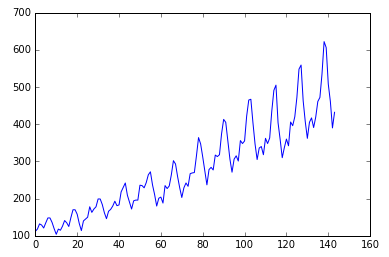
plt.plot(dataset)
plt.show()

The 12-year data show an upward trend, with periodic seasonal patterns for the 12 months of each year.

The data needs to be transformed:

Turn one column into two columns, the first is the number of passengers in month T and the second is the number of passengers in column t+1.
look_back is the time steps needed to predict the next step:

Timsteps is the LSTM's belief that each input data is related to the first number of successive inputs.For example, with segment sequence data like'...ABCDBCEDF..."When timesteps is 3, if the input data is "D" in the model prediction, the predicted output is more likely to be B if the previously received data is "B" and "C", and F if the previously received data is "C" and "E".

# X is the number of passengers at a given time (t) and Y is the number of passengers at the next time (t + 1).

# convert an array of values into a dataset matrix
def create_dataset(dataset, look_back=1):
    dataX, dataY = [], []
    for i in range(len(dataset)-look_back-1):
        a = dataset[i:(i+look_back), 0]
        dataX.append(a)
        dataY.append(dataset[i + look_back, 0])
    return numpy.array(dataX), numpy.array(dataY)

# fix random seed for reproducibility
numpy.random.seed(7)

LSTM is sensitive when the activation function is sigmoid or tanh and data is to be regularized
Set 67% as training data, the rest as test data

# normalize the dataset
scaler = MinMaxScaler(feature_range=(0, 1))
dataset = scaler.fit_transform(dataset)


# split into train and test sets
train_size = int(len(dataset) * 0.67)
test_size = len(dataset) - train_size
train, test = dataset[0:train_size,:], dataset[train_size:len(dataset),:]

Data when X=t and Y=t+1, and the dimension at this time is [samples, features]

# use this function to prepare the train and test datasets for modeling
look_back = 1
trainX, trainY = create_dataset(train, look_back)
testX, testY = create_dataset(test, look_back)

X investing in LSTM needs to have this structure: [samples, time steps, features], so do a transformation

# reshape input to be [samples, time steps, features]
trainX = numpy.reshape(trainX, (trainX.shape[0], 1, trainX.shape[1]))
testX = numpy.reshape(testX, (testX.shape[0], 1, testX.shape[1]))

Establish LSTM model:
There is one input in the input layer and four neurons in the hidden layer. The output layer predicts a value. The activation function is iterated 100 times with sigmoid and batch size is 1.

# create and fit the LSTM network
model = Sequential()
model.add(LSTM(4, input_shape=(1, look_back)))
model.add(Dense(1))
model.compile(loss='mean_squared_error', optimizer='adam')
model.fit(trainX, trainY, epochs=100, batch_size=1, verbose=2)

Epoch 100/100
1s - loss: 0.0020

Forecast:

# make predictions
trainPredict = model.predict(trainX)
testPredict = model.predict(testX)

Convert the predicted data to the same unit before calculating the error

# invert predictions
trainPredict = scaler.inverse_transform(trainPredict)
trainY = scaler.inverse_transform([trainY])
testPredict = scaler.inverse_transform(testPredict)
testY = scaler.inverse_transform([testY])

Calculate mean squared error

trainScore = math.sqrt(mean_squared_error(trainY[0], trainPredict[:,0]))
print('Train Score: %.2f RMSE' % (trainScore))
testScore = math.sqrt(mean_squared_error(testY[0], testPredict[:,0]))
print('Test Score: %.2f RMSE' % (testScore))

Train Score: 22.92 RMSE
Test Score: 47.53 RMSE

Draw the result: blue is the original data, green is the predicted value of the training set, and red is the predicted value of the test set

# shift train predictions for plotting
trainPredictPlot = numpy.empty_like(dataset)
trainPredictPlot[:, :] = numpy.nan
trainPredictPlot[look_back:len(trainPredict)+look_back, :] = trainPredict

# shift test predictions for plotting
testPredictPlot = numpy.empty_like(dataset)
testPredictPlot[:, :] = numpy.nan
testPredictPlot[len(trainPredict)+(look_back*2)+1:len(dataset)-1, :] = testPredict

# plot baseline and predictions
plt.plot(scaler.inverse_transform(dataset))
plt.plot(trainPredictPlot)
plt.plot(testPredictPlot)
plt.show()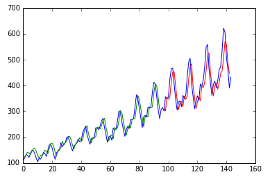

The above results are not optimal, just an example of how LSTM predicts time series
Where can be improved, is it better to have 128 neurons in the most direct hidden layer, 2 or more hidden layers, and 3 time steps?

Another interesting cylinder is whether RNN is good at predicting time series.

Reference material:
http://machinelearningmastery.com/time-series-prediction-lstm-recurrent-neural-networks-python-keras/

Recommended reading
Summary of historical technology blog links
Maybe you can find what you want