brief introduction
Using Pandas's pivot method, DF can be rotated and transformed. This paper will explain the secret of pivot in detail.
Using Pivot
pivot is used to reorganize the DF, and use the specified index, columns and values to reconstruct the existing DF.
Take a Pivot example:

Through pivot change, the new DF uses the value in foo as index, the value of bar as columns and zoo as the corresponding value.
Let's take another example of time change:
In [1]: df
Out[1]:
         date variable     value
0  2000-01-03        A  0.469112
1  2000-01-04        A -0.282863
2  2000-01-05        A -1.509059
3  2000-01-03        B -1.135632
4  2000-01-04        B  1.212112
5  2000-01-05        B -0.173215
6  2000-01-03        C  0.119209
7  2000-01-04        C -1.044236
8  2000-01-05        C -0.861849
9  2000-01-03        D -2.104569
10 2000-01-04        D -0.494929
11 2000-01-05        D  1.071804
In [3]: df.pivot(index='date', columns='variable', values='value')
Out[3]:
variable           A         B         C         D
date
2000-01-03  0.469112 -1.135632  0.119209 -2.104569
2000-01-04 -0.282863  1.212112 -1.044236 -0.494929
2000-01-05 -1.509059 -0.173215 -0.861849  1.071804
If the remaining value is more than one column, each column will have a corresponding column value:
In [4]: df['value2'] = df['value'] * 2

In [5]: pivoted = df.pivot(index='date', columns='variable')

In [6]: pivoted
Out[6]:
               value                                  value2
variable           A         B         C         D         A         B         C         D
date
2000-01-03  0.469112 -1.135632  0.119209 -2.104569  0.938225 -2.271265  0.238417 -4.209138
2000-01-04 -0.282863  1.212112 -1.044236 -0.494929 -0.565727  2.424224 -2.088472 -0.989859
2000-01-05 -1.509059 -0.173215 -0.861849  1.071804 -3.018117 -0.346429 -1.723698  2.143608
By selecting value2, you can get the corresponding subset:
In [7]: pivoted['value2']
Out[7]:
variable           A         B         C         D
date
2000-01-03  0.938225 -2.271265  0.238417 -4.209138
2000-01-04 -0.565727  2.424224 -2.088472 -0.989859
2000-01-05 -3.018117 -0.346429 -1.723698  2.143608
Using Stack
Stack is used to convert DF and convert the column into a new internal index.
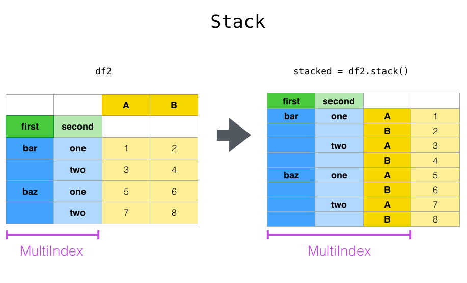
Above, we convert columns A and B to index.
unstack is the reverse operation of stack, which converts the innermost index into the corresponding column.

For example:
In [8]: tuples = list(zip(*[['bar', 'bar', 'baz', 'baz',
   ...:                      'foo', 'foo', 'qux', 'qux'],
   ...:                     ['one', 'two', 'one', 'two',
   ...:                      'one', 'two', 'one', 'two']]))
   ...:

In [9]: index = pd.MultiIndex.from_tuples(tuples, names=['first', 'second'])

In [10]: df = pd.DataFrame(np.random.randn(8, 2), index=index, columns=['A', 'B'])

In [11]: df2 = df[:4]

In [12]: df2
Out[12]:
                     A         B
first second
bar   one     0.721555 -0.706771
      two    -1.039575  0.271860
baz   one    -0.424972  0.567020
      two     0.276232 -1.087401
In [13]: stacked = df2.stack()

In [14]: stacked
Out[14]:
first  second
bar    one     A    0.721555
               B   -0.706771
       two     A   -1.039575
               B    0.271860
baz    one     A   -0.424972
               B    0.567020
       two     A    0.276232
               B   -1.087401
dtype: float64
By default, unstack is the last index of unstack. We can also specify a specific index value:
In [15]: stacked.unstack()
Out[15]:
                     A         B
first second
bar   one     0.721555 -0.706771
      two    -1.039575  0.271860
baz   one    -0.424972  0.567020
      two     0.276232 -1.087401

In [16]: stacked.unstack(1)
Out[16]:
second        one       two
first
bar   A  0.721555 -1.039575
      B -0.706771  0.271860
baz   A -0.424972  0.276232
      B  0.567020 -1.087401

In [17]: stacked.unstack(0)
Out[17]:
first          bar       baz
second
one    A  0.721555 -0.424972
       B -0.706771  0.567020
two    A -1.039575  0.276232
       B  0.271860 -1.087401

By default, stack will only stack one level, and multiple levels can be passed in:
In [23]: columns = pd.MultiIndex.from_tuples([
   ....:     ('A', 'cat', 'long'), ('B', 'cat', 'long'),
   ....:     ('A', 'dog', 'short'), ('B', 'dog', 'short')],
   ....:     names=['exp', 'animal', 'hair_length']
   ....: )
   ....:

In [24]: df = pd.DataFrame(np.random.randn(4, 4), columns=columns)

In [25]: df
Out[25]:
exp                 A         B         A         B
animal            cat       cat       dog       dog
hair_length      long      long     short     short
0            1.075770 -0.109050  1.643563 -1.469388
1            0.357021 -0.674600 -1.776904 -0.968914
2           -1.294524  0.413738  0.276662 -0.472035
3           -0.013960 -0.362543 -0.006154 -0.923061

In [26]: df.stack(level=['animal', 'hair_length'])
Out[26]:
exp                          A         B
  animal hair_length
0 cat    long         1.075770 -0.109050
  dog    short        1.643563 -1.469388
1 cat    long         0.357021 -0.674600
  dog    short       -1.776904 -0.968914
2 cat    long        -1.294524  0.413738
  dog    short        0.276662 -0.472035
3 cat    long        -0.013960 -0.362543
  dog    short       -0.006154 -0.923061
The above is equivalent to:
In [27]: df.stack(level=[1, 2])
Using melt
melt specifies a specific column as a flag variable, and other columns are converted to row data. And placed in two new columns: variable and value.
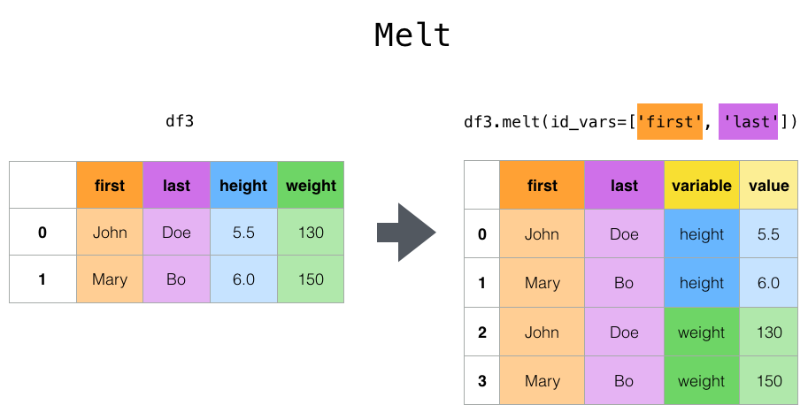
In the above example, we specify two columns, first and last, which are invariant, and height and weight are transformed into row data.
for instance:
In [41]: cheese = pd.DataFrame({'first': ['John', 'Mary'],
   ....:                        'last': ['Doe', 'Bo'],
   ....:                        'height': [5.5, 6.0],
   ....:                        'weight': [130, 150]})
   ....:

In [42]: cheese
Out[42]:
  first last  height  weight
0  John  Doe     5.5     130
1  Mary   Bo     6.0     150

In [43]: cheese.melt(id_vars=['first', 'last'])
Out[43]:
  first last variable  value
0  John  Doe   height    5.5
1  Mary   Bo   height    6.0
2  John  Doe   weight  130.0
3  Mary   Bo   weight  150.0

In [44]: cheese.melt(id_vars=['first', 'last'], var_name='quantity')
Out[44]:
  first last quantity  value
0  John  Doe   height    5.5
1  Mary   Bo   height    6.0
2  John  Doe   weight  130.0
3  Mary   Bo   weight  150.0
Using Pivot tables
Although Pivot can rotate the axis of DF, Pandas also provides pivot_table() can perform numerical statistics while transposing.
pivot_table() receives the following parameters:
data: a df object
values: one or more columns of data to be aggregated.
Index: grouping object of index
Columns: grouping objects for columns
Aggfunc: method of aggregation.
Create a df first:
In [59]: import datetime

In [60]: df = pd.DataFrame({'A': ['one', 'one', 'two', 'three'] * 6,
   ....:                    'B': ['A', 'B', 'C'] * 8,
   ....:                    'C': ['foo', 'foo', 'foo', 'bar', 'bar', 'bar'] * 4,
   ....:                    'D': np.random.randn(24),
   ....:                    'E': np.random.randn(24),
   ....:                    'F': [datetime.datetime(2013, i, 1) for i in range(1, 13)]
   ....:                    + [datetime.datetime(2013, i, 15) for i in range(1, 13)]})
   ....:

In [61]: df
Out[61]:
        A  B    C         D         E          F
0     one  A  foo  0.341734 -0.317441 2013-01-01
1     one  B  foo  0.959726 -1.236269 2013-02-01
2     two  C  foo -1.110336  0.896171 2013-03-01
3   three  A  bar -0.619976 -0.487602 2013-04-01
4     one  B  bar  0.149748 -0.082240 2013-05-01
..    ... ..  ...       ...       ...        ...
19  three  B  foo  0.690579 -2.213588 2013-08-15
20    one  C  foo  0.995761  1.063327 2013-09-15
21    one  A  bar  2.396780  1.266143 2013-10-15
22    two  B  bar  0.014871  0.299368 2013-11-15
23  three  C  bar  3.357427 -0.863838 2013-12-15

[24 rows x 6 columns]
Here are some examples of aggregation:
In [62]: pd.pivot_table(df, values='D', index=['A', 'B'], columns=['C'])
Out[62]:
C             bar       foo
A     B
one   A  1.120915 -0.514058
      B -0.338421  0.002759
      C -0.538846  0.699535
three A -1.181568       NaN
      B       NaN  0.433512
      C  0.588783       NaN
two   A       NaN  1.000985
      B  0.158248       NaN
      C       NaN  0.176180

In [63]: pd.pivot_table(df, values='D', index=['B'], columns=['A', 'C'], aggfunc=np.sum)
Out[63]:
A       one               three                 two
C       bar       foo       bar       foo       bar       foo
B
A  2.241830 -1.028115 -2.363137       NaN       NaN  2.001971
B -0.676843  0.005518       NaN  0.867024  0.316495       NaN
C -1.077692  1.399070  1.177566       NaN       NaN  0.352360

In [64]: pd.pivot_table(df, values=['D', 'E'], index=['B'], columns=['A', 'C'],
   ....:                aggfunc=np.sum)
   ....:
Out[64]:
          D                                                           E
A       one               three                 two                 one               three                 two
C       bar       foo       bar       foo       bar       foo       bar       foo       bar       foo       bar       foo
B
A  2.241830 -1.028115 -2.363137       NaN       NaN  2.001971  2.786113 -0.043211  1.922577       NaN       NaN  0.128491
B -0.676843  0.005518       NaN  0.867024  0.316495       NaN  1.368280 -1.103384       NaN -2.128743 -0.194294       NaN
C -1.077692  1.399070  1.177566       NaN       NaN  0.352360 -1.976883  1.495717 -0.263660       NaN       NaN  0.872482
Adding margins=True will add an All column, indicating that All columns are aggregated:
In [69]: df.pivot_table(index=['A', 'B'], columns='C', margins=True, aggfunc=np.std)
Out[69]:
                D                             E
C             bar       foo       All       bar       foo       All
A     B
one   A  1.804346  1.210272  1.569879  0.179483  0.418374  0.858005
      B  0.690376  1.353355  0.898998  1.083825  0.968138  1.101401
      C  0.273641  0.418926  0.771139  1.689271  0.446140  1.422136
three A  0.794212       NaN  0.794212  2.049040       NaN  2.049040
      B       NaN  0.363548  0.363548       NaN  1.625237  1.625237
      C  3.915454       NaN  3.915454  1.035215       NaN  1.035215
two   A       NaN  0.442998  0.442998       NaN  0.447104  0.447104
      B  0.202765       NaN  0.202765  0.560757       NaN  0.560757
      C       NaN  1.819408  1.819408       NaN  0.650439  0.650439
All      1.556686  0.952552  1.246608  1.250924  0.899904  1.059389
Using crosstab
Crosstab is used to count the number of occurrences of elements in a table.
In [70]: foo, bar, dull, shiny, one, two = 'foo', 'bar', 'dull', 'shiny', 'one', 'two'

In [71]: a = np.array([foo, foo, bar, bar, foo, foo], dtype=object)

In [72]: b = np.array([one, one, two, one, two, one], dtype=object)

In [73]: c = np.array([dull, dull, shiny, dull, dull, shiny], dtype=object)

In [74]: pd.crosstab(a, [b, c], rownames=['a'], colnames=['b', 'c'])
Out[74]:
b    one        two
c   dull shiny dull shiny
a
bar    1     0    0     1
foo    2     1    1     0
The crosstab can receive two Series:
In [75]: df = pd.DataFrame({'A': [1, 2, 2, 2, 2], 'B': [3, 3, 4, 4, 4],
   ....:                    'C': [1, 1, np.nan, 1, 1]})
   ....:

In [76]: df
Out[76]:
   A  B    C
0  1  3  1.0
1  2  3  1.0
2  2  4  NaN
3  2  4  1.0
4  2  4  1.0

In [77]: pd.crosstab(df['A'], df['B'])
Out[77]:
B  3  4
A
1  1  0
2  1  3
You can also use normalize to specify the scale value:
In [82]: pd.crosstab(df['A'], df['B'], normalize=True)
Out[82]:
B    3    4
A
1  0.2  0.0
2  0.2  0.6
You can also normalize rows or columns:
In [83]: pd.crosstab(df['A'], df['B'], normalize='columns')
Out[83]:
B    3    4
A
1  0.5  0.0
2  0.5  1.0
You can specify the aggregation method:
In [84]: pd.crosstab(df['A'], df['B'], values=df['C'], aggfunc=np.sum)
Out[84]:
B    3    4
A
1  1.0  NaN
2  1.0  2.0
get_dummies
get_dummies can convert a column in DF into a combination of 0 and 1 of k columns:
df = pd.DataFrame({'key': list('bbacab'), 'data1': range(6)})

df
Out[9]:
   data1 key
0      0   b
1      1   b
2      2   a
3      3   c
4      4   a
5      5   b

pd.get_dummies(df['key'])
Out[10]:
   a  b  c
0  0  1  0
1  0  1  0
2  1  0  0
3  0  0  1
4  1  0  0
5  0  1  0
get_dummies and cut can be combined to count the elements in the range:
In [95]: values = np.random.randn(10)

In [96]: values
Out[96]:
array([ 0.4082, -1.0481, -0.0257, -0.9884,  0.0941,  1.2627,  1.29  ,
        0.0824, -0.0558,  0.5366])

In [97]: bins = [0, 0.2, 0.4, 0.6, 0.8, 1]

In [98]: pd.get_dummies(pd.cut(values, bins))
Out[98]:
   (0.0, 0.2]  (0.2, 0.4]  (0.4, 0.6]  (0.6, 0.8]  (0.8, 1.0]
0           0           0           1           0           0
1           0           0           0           0           0
2           0           0           0           0           0
3           0           0           0           0           0
4           1           0           0           0           0
5           0           0           0           0           0
6           0           0           0           0           0
7           1           0           0           0           0
8           0           0           0           0           0
9           0           0           1           0           0
get_dummies can also accept a DF parameter:
In [99]: df = pd.DataFrame({'A': ['a', 'b', 'a'], 'B': ['c', 'c', 'b'],
   ....:                    'C': [1, 2, 3]})
   ....:

In [100]: pd.get_dummies(df)
Out[100]:
   C  A_a  A_b  B_b  B_c
0  1    1    0    0    1
1  2    0    1    0    1
2  3    1    0    1    0
This article has been included in http://www.flydean.com/05-python-pandas-reshaping-pivot/
The most popular interpretation, the most profound dry goods, the most concise tutorial, and many tips you don't know are waiting for you to find!
Welcome to my official account: "those things in procedure", understand technology, know you better!