Alex's alexnet network structure model won the championship in Imagenet 2012 image classification challenge. When training alexnet, the author cycled the training set of 1.2 million images for 90 times, and spent five to six days on two NVIDIA GTX 580 3gb GPUs.
Source paper: Krizhevsky, Alex, Ilya Sutskever, and Geoffrey E. Hinton. "Imagenet classification with deep convolutional neural networks." Advances in neural information processing systems. 2012."
I. innovations of AlexNet:
1 replace the previous sigmoid with Relu as the activation function
2 Data Augmentation strategy is used to suppress over fitting
3 uses overlapping Max Pooling. Previously, CNN usually used average pooling, while AlexNet used maximum pooling, which successfully avoided the blurring effect caused by average pooling
4 propose LRN (local response normalization)
5. Dropout mechanism was successfully used to suppress overfitting
6 multi GPU training
Details are as follows:
1 ReLu as activation function
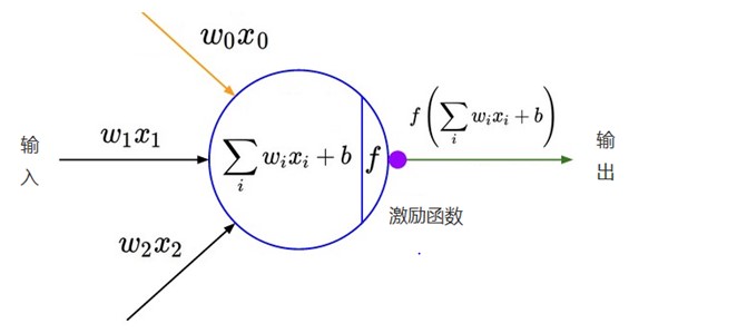
In the initial perceptron model, the relationship between input and output is as follows:
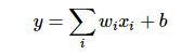
Only a simple linear relationship, such a network structure has great limitations: that is, using many network layers with such a structure, its output and input are still linear, and can not deal with the input and output with nonlinear relationship. Therefore, make a nonlinear conversion to the output of each neuron, that is, input the above weighted sum result into a nonlinear function, that is, the activation function. In this way, due to the introduction of activation function, the superposition of multiple network layers is no longer a simple linear transformation, but has stronger performance ability. Initially, sigmoid and tanh functions were the most commonly used activation functions.
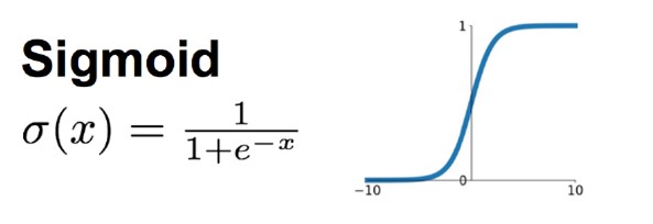
**Sigmoid: * * when the number of network layers is small, the characteristics of sigmoid function can well meet the role of activation function. It compresses a real number between 0 and 1. When the input number is very large, the result will be close to 1; When you enter a very large negative number, you get a result close to 0. This characteristic can well simulate whether neurons are activated and transmit information back after stimulation (output is 0, almost not activated; output is 1, completely activated).
A big problem with sigmoid is gradient saturation. Observe the curve of sigmoid function. When the input number is large (or small), its function value tends to remain unchanged and its derivative becomes very small. In this way, in the network structure with many layers, the result tends to zero and the weight update is slow due to the accumulation of many small sigmoid derivatives during back propagation.
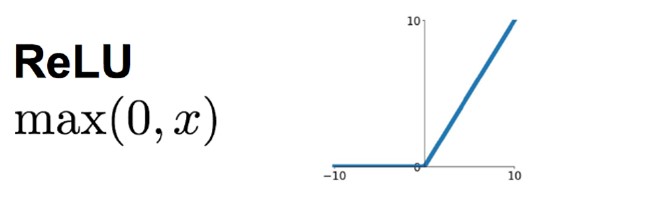
**ReLU: * * to solve the problem of slow training convergence caused by sigmoid gradient saturation, ReLU is introduced into AlexNet. ReLU is a piecewise linear function. If it is less than or equal to 0, the output is 0; If it is greater than 0, the identity output. Compared with sigmoid, ReLU has the following characteristics:
(1) Low computational overhead. The forward propagation of sigmoid has exponential operation and reciprocal operation, while relu is linear output; In back propagation, sigmoid has exponential operation, while relu has output part, and the derivative is always 1.
(2) Gradient saturation problem
(3) Sparsity. Relu will make the output of some neurons 0, which leads to the sparsity of the network, reduces the interdependence of parameters and alleviates the occurrence of over fitting problem.
There is a problem here. As mentioned earlier, the activation function should be nonlinear in order to make the network structure have stronger expression ability. The use of ReLU here is essentially a linear piecewise function, how to carry out nonlinear transformation.
Here, the neural network is regarded as A huge transformation matrix M, whose input is matrix A composed of all training samples and output is matrix B. If m here is A linear transformation, then all training samples A are linearly transformed and output as B.

Then, for ReLU, because it is segmented, the part of 0 can be regarded as that neurons are not activated. Different neurons are activated or inactive, and the transformation matrix composed of neurons is different.
There are two training samples A1 and A2, and the transformation matrix composed of neural network during training is M1 and M2. Since the activated neurons in the neural network corresponding to M1 transformation are different from m2, M1 and M2 are actually two different linear transformations. In other words, the linear transformation matrix Mi used by each training sample is different. In the whole training sample space, it experiences nonlinear transformation.
In short, the same features in different training samples will flow through different neurons during neural network learning (neurons with activation function value of 0 will not be activated). In this way, the final output is actually the nonlinear transformation of the input sample. A single training sample is a linear transformation, but the linear transformation of each training sample is different, so the whole training sample set is a nonlinear transformation.
The traditional neural network activation function is usually arctangent or sigmoid. AlexNet uses RELU as the activation function. Compared with inverse tangent, the training speed of this method is about 6 times higher. The RELU activation function is incredibly simple.
2 data enhancement
Because of many training parameters, neural network needs more data, otherwise it is easy to over fit. When the training data is limited, some new data can be generated from the existing training data set through some transformations to quickly expand the training data. For the image data set, some deformation operations can be performed on the image:
(1) Flip
(2) Random clipping
(3) Translation, transformation of color illumination
The following operations are performed on the data in AlexNet:
(1) Random clipping, pair 256 × 256 pictures are randomly cropped to 227 × 227, and then flip horizontally.
(2) During the test, cut the upper left, upper right, lower left, lower right and middle for 5 times respectively, and then turn them over for a total of 10 cuts, and then average the results.
(3) PCA (principal component analysis) is used for RGB channels. For each pixel of each training image, the feature vectors and eigenvalues of three RGB channels are extracted, and each eigenvalue is multiplied by one α,α It is a random variable whose mean value is 0.1 and variance obeys Gaussian distribution. That is, the color and illumination are changed, and the error rate is reduced by 1%.
3. Cascade pooling
In LeNet, pooling does not overlap, that is, the size and step size of the pooled window are the same, as follows:
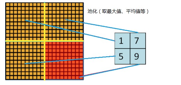
The Pooling used in AlexNet can be overlapped, that is, when Pooling, the step size of each move is less than the length of the pooled window. The size of the AlexNet pool is 3 × 3 square, and the step length of each pool movement is 2, so there will be overlap. Overlapping Pooling can avoid over fitting, and this strategy contributes 0.3% of the Top-5 error rate. Compared with the non overlapping scheme s=2, z=2s=2, z=2, the output dimensions are equal, and the over fitting can be suppressed to a certain extent.
4 local response normalization
ReLU has satisfactory characteristics. It does not need input normalization to prevent saturation. If at least some training samples produce positive input to ReLU, then that neuron will learn. However, we still find that the following local response normalization contributes to generalization. a(x,y)(i) represents neuronal activation. It is calculated by applying nuclear i at position (x,y) and then applying ReLU nonlinearity. The response normalized activation b(x,y)(i) is given by the following formula:
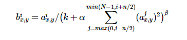
Where n is the number of convolution kernels, that is, the number of generated featuremaps; k, α,β, N is a super parameter. The values used in this paper are k = 2 and N = 5, α= 10(-4), β= 0.75.
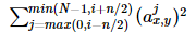
The superscript of output b(x,y)(i) and input a(x,y)(j) indicates the channel where the current value is located, that is, the direction of superposition is along the channel. Add up the squares of the values at the same position of the channel near the value a(x,y)(i) to be normalized
Hinton et al. Believe that LRN layer imitates the lateral inhibition mechanism of biological nervous system and creates a competition mechanism for the activities of local neurons, so that the value with large response is relatively larger and improves the generalization ability of the model. However, later papers, such as very deep revolution networks for large-scale image recognition (that is, the article proposing VGG network), proved that LRN has no effect on CNN, but increases the computational complexity. Therefore, this technology is no longer used.
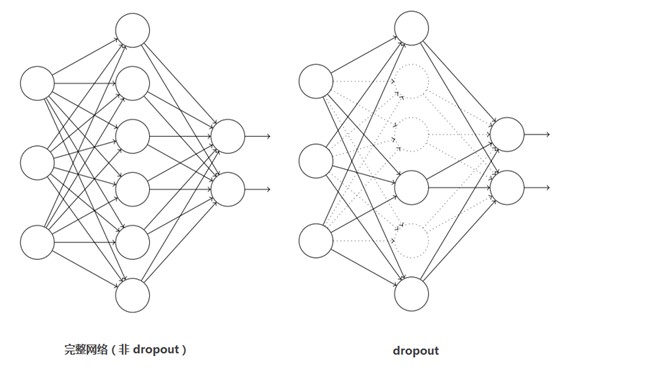
5 Dropout
This is a commonly used method to suppress over fitting.
Dropout is mainly introduced to prevent over fitting. In the neural network, dropout is realized by modifying the structure of the neural network itself. For the neuron of a certain layer, set the neuron to 0 through the defined probability, and the neuron will not participate in the forward and backward propagation, just like being deleted in the network, while keeping the number of neurons in the input layer and the output layer unchanged, Then the parameters are updated according to the learning method of neural network. In the next iteration, some neurons are randomly deleted again (set to 0) until the end of training.
Dropout should be regarded as a great innovation in AlexNet, and now it is one of the necessary structures in neural network. Dropout can also be regarded as a kind of model combination. The network structure generated each time is different. The over fitting can be effectively reduced by combining multiple models. Dropout only needs twice the training time to realize the effect of model combination (similar to averaging), which is very efficient.
As shown below:
In AlexNet, keep of each layer during training_ Prob is set to 0.5, while during the test, all keep_ The prob is 1.0, that is, turn off dropout, and multiply the output of all neurons by 0.5 to ensure that the average output during training and testing is close. Of course, dropout is only used for the full connection layer. Without dropout, AlexNet network will encounter serious over fitting. After joining dropout, the convergence speed of the network is nearly doubled.
II. AlexNet network structure
AlexNet and LeNet-5-networks are slightly different. In LeNet-5 network, convolution layer and pooling layer are separated, that is, one convolution layer and one pooling layer are distributed in this way. However, AlexNet network convolution and pooling layer are integrated, and the network is designed in two ways.
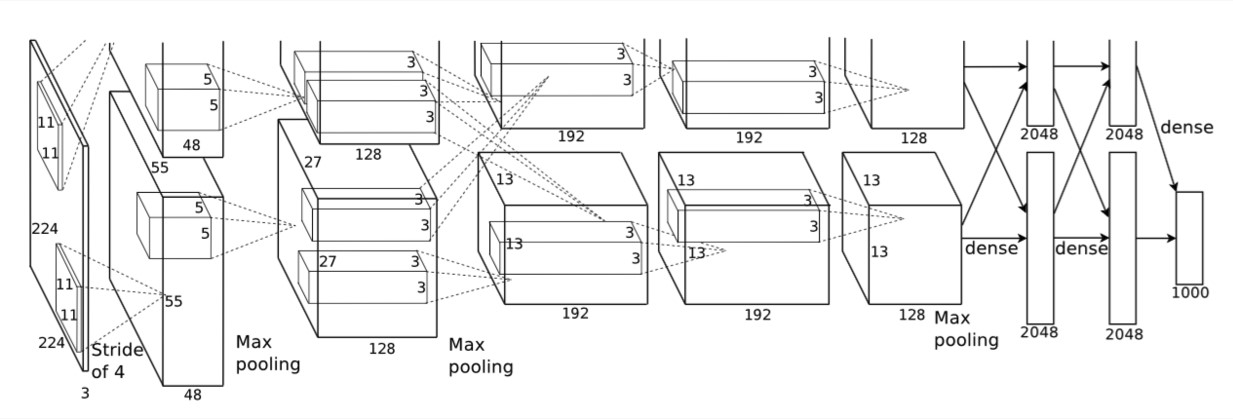
(1) In general:
(1) AlexNet is an 8-layer structure, in which the first 5 layers are convolution layers and the last 3 layers are full connection layers; There are 60 million learning parameters and 650000 neurons.
(2) AlexNet runs on two GPU s.
(3) In layers 2, 4 and 5, AlexNet is connected in its own GPU of the previous layer, and layer 3 is fully connected with the previous two layers. The full connection is the full connection of two GPUs.
(4) After the 1st and 2nd convolution layers of LRN layer.
(5) The Max pooling layer is behind the LRN layer and the fifth convolution layer.
(6) ReLU is behind each convolution layer and full connection layer.
(7) The Dropout layer reduces overfitting and is applied to the first two fully connected layers.
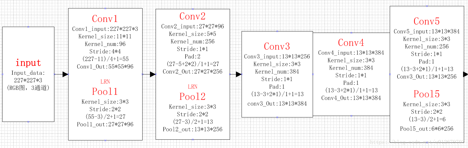
(2) Explain the calculation of training parameters of each layer in detail:
The first five layers: convolution layer
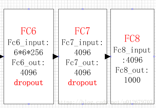
The last three floors: full connection floor
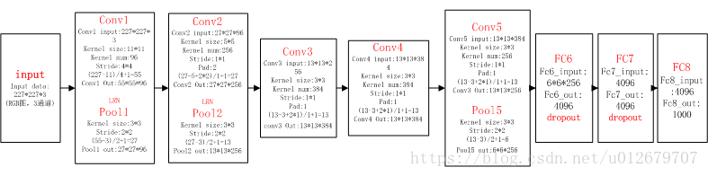
Overall calculation diagram:
(3) Explain each layer of AlexNet network in detail:
Convolution layer C1
The processing flow of this layer is: convolution – > relu – > pooling – > normalization.
(1) Convolution, the input is 227 × 227 * 3, using 96 11 × eleven × 3 (the dimension of the last convolution kernel must be the same as the dimension of the last input kernel), and the obtained FeatureMap is 55 × fifty-five × 96.
(2) ReLU, input the FeatureMap output by the convolution layer into the ReLU function.
(3) Pooling, using 3 × 3 pool cells with step size of 2 (overlapping pool, step size is less than the width of pool cells), and the output is 27 × twenty-seven × 96((55−3)/2+1=27.
(4) Local response normalization, using k=2,n=5, α= 10(−4), β= 0.75 for local normalization, the output is still 27 × twenty-seven × 96. The output is divided into two groups, with the size of each group being 27 × twenty-seven × 48.
Convolution layer C2
The processing flow of this layer is: convolution – > relu – > pooling – > normalization
(1) Convolution, input is 2 groups 27 × twenty-seven × 48. Use 2 groups, 128 in each group, size 5 × five × 48, and the edge filling is made. padding=2, and the step size of convolution is 1 Then the output FeatureMap is 2 groups, and the size of each group is 27 × 27 times128. ((27+2∗2−5)/1+1=27
(2) ReLU, input the FeatureMap output by the convolution layer into the ReLU function.
(3) The size of pooling operation is 3 × 3. The step size is 2, the size of the pooled image is (27 − 3) / 2 + 1 = 13, and the output is 13 × thirteen × 256.
(4) Local response normalization, using k=2,n=5, α= 10(−4), β= 0.75 for local normalization, the output is still 13 × thirteen × 256, the output is divided into 2 groups, and the size of each group is 13 × thirteen × 128.
Convolution layer C3
The processing flow of this layer is: convolution – > relu
(1) Convolution, input is 13 × thirteen × 256, using 2 groups of 384, size 3 × three × 256 convolution kernel with edge padding=1 and convolution step size of 1. Then the output FeatureMap is 13 × thirteen × 384.
(2) ReLU, input the FeatureMap output by the convolution layer into the ReLU function.
Convolution layer C4
The processing flow of this layer is: convolution – > relu
This layer is similar to C3.
(1) Convolution, input is 13 × thirteen × 384, divided into two groups, 13 in each group × thirteen × 192. Use 2 groups, 192 in each group, size 3 × three × The convolution kernel of 192 is filled with edges, padding=1, and the step size of convolution is 1. Then the output FeatureMap is 13 × 13 times384, divided into two groups, with 13 in each group × thirteen × 192.
(2) ReLU, input the FeatureMap output by the convolution layer into the ReLU function.
Convolution layer C5
The processing flow of this layer is: convolution – > relu – > pooling
(1) Convolution, input 13 × thirteen × 384, divided into two groups, 13 in each group × thirteen × 192. Use 2 groups with 128 in each group and 3 in size × three × The edge of the convolution kernel is padded to 192. Then the output FeatureMap is 13 × thirteen × 256.
(2) ReLU, input the FeatureMap output by the convolution layer into the ReLU function.
(3) Pool, the size of pool operation is 3 × 3. The step size is 2. The size of the pooled image is (13 − 3) / 2 + 1 = 6, that is, the output after pooling is 6 × six × 256.
Full connection layer FC6
The flow of this layer is: (convolution) full connection -- > relu -- > dropout
(1) Convolution - > full connection: the input is 6 × six × 256. There are 4096 convolution cores in this layer, and the size of each convolution core is 6 × six × 256. Since the size of the convolution kernel is just the same as that of the feature map (input) to be processed, that is, each coefficient in the convolution kernel is multiplied by only one pixel value of the feature map (input) size and corresponds one by one, this layer is called the full connection layer. Because the size of convolution kernel is the same as that of characteristic image, there is only one value after convolution operation. Therefore, the size of pixel layer after convolution is 4096 × one × 1, 4096 neurons.
(2) ReLU, the 4096 operation results generate 4096 values through the ReLU activation function.
(3) Dropout, which inhibits over fitting, randomly disconnects some neurons or does not activate some neurons.
Full connection layer FC7
The process is: full connection – > relu – > dropout
(1) Full connection, input vector of 4096.
(2) ReLU, the 4096 operation results generate 4096 values through the ReLU activation function.
(3) Dropout, which inhibits over fitting, randomly disconnects some neurons or does not activate some neurons.
Output layer
4096 data output from the seventh layer are fully connected with 1000 neurons in the eighth layer, and 1000 float type values are output after training, which is the prediction result.
Number of AlexNet parameters
Parameters of convolution layer = number of convolution kernels * convolution kernels + bias
C1: 96 11 × eleven × Convolution kernel of 3, 96 × eleven × eleven × 3+96=34848
C2: 2 groups, 128 in each group, 5 × five × 48 convolution kernel, (128 × five × five × 48+128) × 2=307456
C3: 384 3 × three × 256 convolution kernel, 3 × three × two hundred and fifty-six × 384+384=885120
C4: 2 groups, 192 in each group 3 × three × 192 convolution kernel, (3 × three × one hundred and ninety-two × 192+192) × 2=663936
C5: 2 groups, 128 in each group, 3 × three × 192 convolution kernel, (3 × three × one hundred and ninety-two × 128+128) × 2=442624
FC6: 4096 6 × six × 256 convolution kernel, 6 × six × two hundred and fifty-six × 4096+4096=37752832
FC7: 4096∗4096+4096=16781312
output: 4096∗1000=4096000
The convolution kernels in convolution layers C2, C4 and C5 are only connected to the FeatureMap on the upper layer of the same GPU. As can be seen from the above, most parameters are concentrated in the full connection layer, and there are few weight parameters in the convolution layer due to weight sharing.
(4) Details of Learning
(1) The input is 224 × two hundred and twenty-four thousand two hundred and twenty-four × 224, but after calculation (224 − 11) / 4 = 54.75 is not 55 in the paper × 55 instead of 227 × 227 as input, then (227 − 11) / 4 = 55.
(2) The pixels of the input picture are 224x224 and have three layers, which represent the three primary colors RGB (we know that the so-called color is actually composed of the three primary colors, so the color picture is the same). We can simply see it as a color picture composed of three stacked pictures, which correspond to red, green and blue respectively. There is only one layer in the lenet-5-network, Because the color is gray. The sampling window of the input layer is 11 × 11 and there are three layers corresponding to the three layers of the picture. How many connections are there for each sampling? There are 11x11x3 = 363, and the translation step size of the sampling window is 4. (in lenet-5-network, the mobile step size is 1, here is 4, which should be easy to understand). Why is the step size 4 instead of 1? Considering the amount of calculation, the amount of calculation in step 1 is too large. So what is the dimension of such a sampling window after sampling on the image?
(3) AlexNet uses Mini batch SGD, the size of batch is 128, the gradient descent algorithm selects momentum, the parameter is 0.9, L2 regularization or weight attenuation is added, and the parameter is 0.0005. It is mentioned in the paper that such a small weight attenuation parameter has almost no regularization effect, but it is very important for model learning.
(4) The weight of each layer is initialized to the Gaussian distribution of 0 mean and 0.01 standard deviation. The offset of convolution in the second, fourth and fifth layers is set to 1.0, while that in other layers is 0, in order to accelerate the rate of early learning (because the activation function is ReLU, the offset of 1.0 can make most of the output positive).
(5) An equal learning rate is used for all layers, which is manually adjusted throughout the training process. The initial value of learning rate is 0.01, which is reduced three times before the end of training. Each reduction occurs when the error rate stops reducing. Each reduction is to divide the learning rate by 10.
(6) Depth is very important. If any layer is removed, the performance will be reduced.
(7) To simplify the experiment, unsupervised pre training was not used. However, when there is enough computing power to expand the network structure without adding corresponding data, unsupervised pre training may be helpful.
Three code implementation (pytoch)
Main reference https://www.bilibili.com/video/BV1W7411T7qc
This part builds the AlexNet network and trains the flower classification data set.
1. Data set download.
http://download.tensorflow.org/example_images/flower_photos.tgz
It contains 5 types of flowers, with 600 ~ 900 images of each type. Set flower_ Copy photos to flower_data folder and unzip it.
2 divide the data set into training set and verification set.
Since this data set is not divided into training set and test set when downloading as CIFAR10, it needs to be divided by itself. split_data.py will divide the data set into training set and verification set according to the ratio of 9:1.
In split_ data. The current page of python, shift + right-click to open the PowerShell window, and enter python split_data.py, it will be converted automatically.
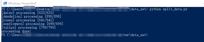
The data set directory after division is as follows:
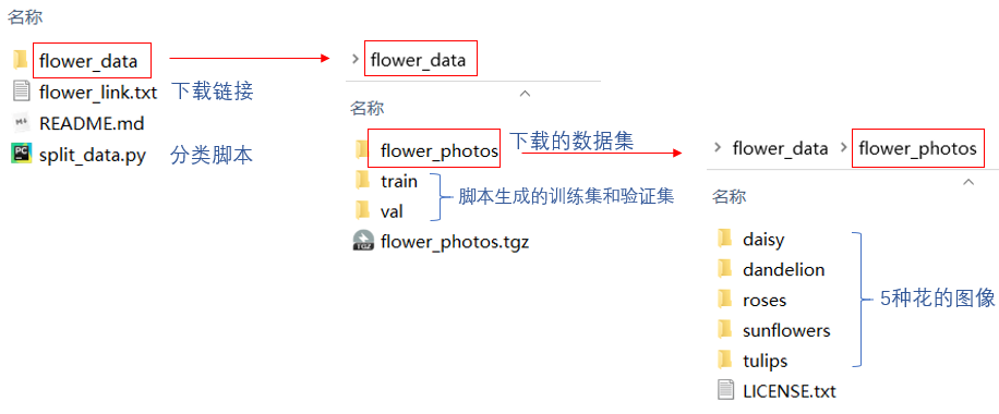
|-- flower_data
	|-- flower_photos
		|-- daisy
		|-- dandelion
		|-- roses
		|-- sunflowers
		|-- tulips
		|-- LICENSE.txt
	|-- train
		|-- daisy
		|-- dandelion
		|-- roses
		|-- sunflowers
		|-- tulips
	|-- val
		|-- daisy
		|-- dandelion
		|-- roses
		|-- sunflowers
		|-- tulips
	|-- flower_photos.tgz
|-- flower_link.txt
|-- README.md
|-- split_data.py
3 note model py.
import torch.nn as nn
import torch

class AlexNet(nn.Module):
    def __init__(self, num_classes=1000, init_weights=False):
        super(AlexNet, self).__init__()
        #Different from LeNet
        #Use NN Sequential module can package a series of layer structures and combine them into a new structure, which is called features here
        self.features = nn.Sequential(
            #padding can be passed into shaping or tuple(1,2). If the integer 1 is passed in, a row of zeros will be filled in the upper and lower parts of the characteristic matrix, and a column of zeros will be filled in the left and right sides.
            # tuple(1,2) means that one row of zeros is filled up and down, and two columns of zeros are filled up on the left and right sides
            #If you want to be more precise, you need to use NN on the official website Zeropad2d ((1,2,1,2)), one column on the left, two columns on the right, one row above and two rows below
            nn.Conv2d(3, 48, kernel_size=11, stride=4, padding=2),  # input[3, 224, 224]  output[48, 55, 55]
            nn.ReLU(inplace=True),
            nn.MaxPool2d(kernel_size=3, stride=2),                  # output[48, 27, 27]
            nn.Conv2d(48, 128, kernel_size=5, padding=2),           # output[128, 27, 27]
            nn.ReLU(inplace=True),
            nn.MaxPool2d(kernel_size=3, stride=2),                  # output[128, 13, 13]
            nn.Conv2d(128, 192, kernel_size=3, padding=1),          # output[192, 13, 13]
            nn.ReLU(inplace=True),
            nn.Conv2d(192, 192, kernel_size=3, padding=1),          # output[192, 13, 13]
            nn.ReLU(inplace=True),
            nn.Conv2d(192, 128, kernel_size=3, padding=1),          # output[128, 13, 13]
            nn.ReLU(inplace=True),
            nn.MaxPool2d(kernel_size=3, stride=2),                  # output[128, 6, 6]
        )
        #It includes three full connection layers
        self.classifier = nn.Sequential(
            #dropout method can inactivate the neurons in the whole connecting layer in a certain proportion to prevent over fitting
            nn.Dropout(p=0.5),
            nn.Linear(128 * 6 * 6, 2048),
            nn.ReLU(inplace=True),
            nn.Dropout(p=0.5),
            nn.Linear(2048, 2048),
            nn.ReLU(inplace=True),
            #The input is the output of the upper layer, and the output is the number of data set categories. There are 5 kinds of flowers here
            #num_ Classes are passed in when initializing classes, def__ init__ (self, num_classes=1000, init_weights=False)
            #Default num_classes=1000. Here are five categories. Just pass in 5 during initialization
            nn.Linear(2048, num_classes),
        )
        #Initialize weight
        #In the process of building a network, when initializing classes, def__ init__ (self, num_classes=1000, init_weights=False):
        #If the passed in parameter init_weights=True, the weights are initialized
        #Here is a method to initialize the weight, but it is not needed. Pytorch will automatically initialize the weight of volume base layer and full connection layer
        if init_weights:
            self._initialize_weights()

    def forward(self, x):
        x = self.features(x)
        #Flattening: the flattening dimension starts from the 1st dimension and the batch does not move in the 0th dimension
        #Starting from the first dimension, C*H*W develops into a one-dimensional vector
        x = torch.flatten(x, start_dim=1)
        x = self.classifier(x)
        return x

    def _initialize_weights(self):
        #Traverse all modules in the network, that is, each layer structure defined will be iterated
        for m in self.modules():
            #Judge the type of the obtained layer structure, if it is NN Conv2d type
            if isinstance(m, nn.Conv2d):
                #Kaiming in this way_ normal_, Initialize weights
                nn.init.kaiming_normal_(m.weight, mode='fan_out', nonlinearity='relu')
                if m.bias is not None:
                    nn.init.constant_(m.bias, 0)
            #If the incoming instance is the full connection layer, through the normal distribution normal_, Assign a value to the weight. The mean of normal distribution is 0 and the variance is 0.01
            elif isinstance(m, nn.Linear):
                nn.init.normal_(m.weight, 0, 0.01)
                nn.init.constant_(m.bias, 0)
4 note train py.
import os
import sys
import json
import torch
import torch.nn as nn
from torchvision import transforms, datasets, utils
import matplotlib.pyplot as plt
import numpy as np
import torch.optim as optim
from tqdm import tqdm
from model import AlexNet
import time
def main():
#Specify the equipment to use in your workout
device = torch.device("cuda:0" if torch.cuda.is_available() else "cpu")
print("using {} device.".format(device))
#Data preprocessing, transforms Randomresizedcrop (224) is randomly cropped to the size of 224 * 224
#transforms.RandomHorizontalFlip() randomly flips horizontally
#To Tensor() to Tensor
#Normalize ((0.5, 0.5, 0.5), (0.5, 0.5))
data_transform = {
"train": transforms.Compose([transforms.RandomResizedCrop(224),
transforms.RandomHorizontalFlip(),
transforms.ToTensor(),
transforms.Normalize((0.5, 0.5, 0.5), (0.5, 0.5, 0.5))]),
"val": transforms.Compose([transforms.Resize((224, 224)), # cannot 224, must (224, 224)
transforms.ToTensor(),
transforms.Normalize((0.5, 0.5, 0.5), (0.5, 0.5, 0.5))])}
#Gets the root directory where the dataset is located
#os.getcwd() gets the directory where the current file is located
#os.path.join(os.getcwd(), "../..") Set OS Getcwd() and ".. /.." The two paths are connected together, ".." Indicates to return to the previous directory
#"../.." Indicates that the upper level directory is returned
data_root = os.path.abspath(os.path.join(os.getcwd(), "../..")) # get data root path
image_path = os.path.join(data_root, "data_set", "flower_data") # flower data set path
assert os.path.exists(image_path), "{} path does not exist.".format(image_path)
#Load training set data set, root = OS path. Join (image_path, "train") is the path to load the training set data set
train_dataset = datasets.ImageFolder(root=os.path.join(image_path, "train"),
transform=data_transform["train"])
#How many pictures are there in the statistical training set
train_num = len(train_dataset)
# {'daisy':0, 'dandelion':1, 'roses':2, 'sunflower':3, 'tulips':4}
#Gets the index corresponding to the name of the classification
#class_to_idx is a dictionary that contains the index value corresponding to each category. You can set a breakpoint to have a look
flower_list = train_dataset.class_to_idx
#Traverse the dictionary and reverse the key and value of the dictionary
cla_dict = dict((val, key) for key, val in flower_list.items())
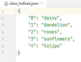
# write dict into json file
#For cla_dict encodes the dictionary into json format
json_str = json.dumps(cla_dict, indent=4)
#Open class_indices.json file, saving information
with open('class_indices.json', 'w') as json_file:
json_file.write(json_str)
batch_size = 32
nw = min([os.cpu_count(), batch_size if batch_size > 1 else 0, 8]) # number of workers
print('Using {} dataloader workers every process'.format(nw))
#Train the training set through DataLoader_ Load the dataset according to batch_size and random parameters to randomly obtain batches of data from samples
#num_workers indicates the number of threads used to load data. Under windows system, it cannot be set to non-zero value
#num_workers=0 means that a main thread is used to load data
train_loader = torch.utils.data.DataLoader(train_dataset,
batch_size=batch_size, shuffle=True,
num_workers=nw)
validate_dataset = datasets.ImageFolder(root=os.path.join(image_path, "val"),
transform=data_transform["val"])
val_num = len(validate_dataset)
validate_loader = torch.utils.data.DataLoader(validate_dataset,
batch_size=batch_size, shuffle=False,
num_workers=nw)
print("using {} images for training, {} images for validation.".format(train_num,
val_num))
#The commented out part is the code for how to view the dataset
#You can put it first validate_loader Inside batch_size Change to 4 # #val_num))
#shuffle=False means random disorder. Change it to shuffle=True, otherwise it will be the same folder and type if it is read in order
# test_data_iter = iter(validate_loader)
# test_image, test_label = test_data_iter.next()
#
# def imshow(img):
# img = img / 2 + 0.5 # unnormalize
# npimg = img.numpy()
# plt.imshow(np.transpose(npimg, (1, 2, 0)))
# plt.show()
#
# print(' '.join('%5s' % cla_dict[test_label[j].item()] for j in range(4)))
# imshow(utils.make_grid(test_image))
net = AlexNet(num_classes=5, init_weights=True)
net.to(device)
#Loss function, multi category loss, cross entropy function
loss_function = nn.CrossEntropyLoss()
# pata = list(net.parameters())
#Adam optimizer is adopted, and the optimization object is all trainable parameters in the network parameters()
#lr=0.0002. The learning rate is obtained in the experiment. The influence of turning up and down on the accuracy can be seen
optimizer = optim.Adam(net.parameters(), lr=0.0002)
epochs = 10
#Path to save weights
save_path = './AlexNet.pth'
#Define the best accuracy. In order to save the training model with the highest accuracy in the process of training the network
best_acc = 0.0
train_steps = len(train_loader)
#Let's start training
for epoch in range(epochs):
# train
net.train()#Enable dropout method
running_loss = 0.0#Statistics of average loss during training
#Count the time required to train an epoch
t1=time.perf_counter()
train_bar = tqdm(train_loader, file=sys.stdout)
#Traversal data set
for step, data in enumerate(train_bar):
#Divide the data into corresponding images and labels
images, labels = data
#Clear previous gradient information
optimizer.zero_grad()
outputs = net(images.to(device))
#Calculate the loss between the predicted value and the real value
loss = loss_function(outputs, labels.to(device))
loss.backward()
optimizer.step()
# print statistics
running_loss += loss.item()
train_bar.desc = "train epoch[{}/{}] loss:{:.3f}".format(epoch + 1,
epochs,
loss)
#Use * and Print the training progress. rate is the training progress
print()
print(time.perf_counter()-t1)
# validate
net.eval()#Close dropout method
acc = 0.0 # accumulate accurate number / epoch
with torch.no_grad():#Loss gradients are not calculated during validation
val_bar = tqdm(validate_loader, file=sys.stdout)
#Traversal validation set
for val_data in val_bar:
#Divide the data into corresponding pictures and labels
val_images, val_labels = val_data
outputs = net(val_images.to(device))
#Through torch Max finds the most likely category in the output
predict_y = torch.max(outputs, dim=1)[1]
#Compare the predicted value with the real label Orch eq(predict_y, val_labels.to(device))
#acc cumulative validation set predicts the number of correct samples
acc += torch.eq(predict_y, val_labels.to(device)).sum().item()
#Accuracy of validation set
val_accurate = acc / val_num
print('[epoch %d] train_loss: %.3f val_accuracy: %.3f' %
(epoch + 1, running_loss / train_steps, val_accurate))
if val_accurate > best_acc:
best_acc = val_accurate
#Save current weights
torch.save(net.state_dict(), save_path)
print('Finished Training')
if __name__ == '__main__':
main()
class_indices.json file:
5 note predict py.
import os
import json

import torch
from PIL import Image
from torchvision import transforms
import matplotlib.pyplot as plt

from model import AlexNet


def main():
    device = torch.device("cuda:0" if torch.cuda.is_available() else "cpu")

    data_transform = transforms.Compose(
        [transforms.Resize((224, 224)),
         transforms.ToTensor(),
         transforms.Normalize((0.5, 0.5, 0.5), (0.5, 0.5, 0.5))])

    # load image
    img_path = "../tulip.jpg"
    assert os.path.exists(img_path), "file: '{}' dose not exist.".format(img_path)
    img = Image.open(img_path)

    plt.imshow(img)
    # [N, C, H, W]
    img = data_transform(img)
    # expand batch dimension
    #Expand one dimension, because the read image has only three dimensions: height, width and depth
    img = torch.unsqueeze(img, dim=0)

    # read class_indict

    json_path = './class_indices.json'
    assert os.path.exists(json_path), "file: '{}' dose not exist.".format(json_path)

    json_file = open(json_path, "r")
    # Read the category name corresponding to the index, decode it and decode it into a dictionary to be used
    class_indict = json.load(json_file)

    # create model
    model = AlexNet(num_classes=5).to(device)#Initialize network

    # load model weights
    weights_path = "./AlexNet.pth"
    assert os.path.exists(weights_path), "file: '{}' dose not exist.".format(weights_path)
    #Load network model
    model.load_state_dict(torch.load(weights_path))

    model.eval()#Turn off dropout mode
    with torch.no_grad():#pytorch does not track the loss gradient of variables
        # predict class
        #The data is propagated forward to get the output, and then the output is compressed to compress the batch dimension
        output = torch.squeeze(model(img.to(device))).cpu()
        #After being processed by softmax, it becomes a probability distribution
        predict = torch.softmax(output, dim=0)
        #Through torch Argmax method to obtain the index value corresponding to the place with the maximum probability
        predict_cla = torch.argmax(predict).numpy()
    #However, due to the category name and its corresponding category probability
    print_res = "class: {}   prob: {:.3}".format(class_indict[str(predict_cla)],
                                                 predict[predict_cla].numpy())
    plt.title(print_res)
    for i in range(len(predict)):
        print("class: {:10}   prob: {:.3}".format(class_indict[str(i)],
                                                  predict[i].numpy()))
    plt.show()


if __name__ == '__main__':
    main()
6. Various problems during program operation.
(1) python package tqdm (progress bar) installation
conda install -c conda-forge tqdm
(2) loss changes during deep learning training
Reference to the following https://blog.csdn.net/qq_42363032/article/details/122489704
**Data set description**
**Training set**It is a sample set used for model training to determine the weight parameters of the model.
The number of training sets increases with the complexity of the model.
Back propagation determines the optimal parameters.
**Validation set**It is used to verify the evaluation of the model, the selection of the model and the adjustment of parameters.
Preliminary model selection and evaluation.
**Test set**It is an unbiased estimation for the model.
Find another set evaluation model to see if it is accidental stability, that is, to verify unbiased.
To ensure the same distribution, it is best to ensure that the positive and negative ratio of the test set is consistent with the actual environment.
If the model performs well in the training set, verification set and test set, but performs poorly in the actual new data, the possible problems are as follows:
The distribution is inconsistent, there are differences between the characteristics of new data and original data, and the network has insufficient ability to extract the characteristics of new data.

**loss explain**
train loss decline↓,val loss decline ↓: Training is normal, the network is still learning, at best.
train loss decline ↓,val loss: rise/Unchanged: a little over fitting overfitting,You can stop training and use fitting methods such as data enhancement, regularization dropout,max pooling Wait.
train loss stable, val loss Descending: if there is a problem with the data, check whether the data is marked incorrectly, whether the distribution has been continuous, and whether the shuffle.
train loss stable, val loss Stable: if the learning process encounters a bottleneck, you can try to reduce the learning rate or batch quantity
train loss rise ↑,val loss rise ↑: Improper network structure design, unreasonable parameters, data sets need to be cleaned, etc.

**loss shock**
Slight shock is normal, within a certain range, generally speaking batch size The larger the, the more accurate the descending direction is, and the smaller the training shock. If the shock is very violent, it is estimated to be batch size The setting is too small.

**train loss Down, val loss rise
 Solution of network over fitting**
Learning rate attenuation
dropout
 Reduce the number of layers and neurons
 plus BN
Early Stopping,Can let val loss Stop early when there is an upward trend
**loss rise, acc Also rise**
If val loss Steady, you can continue training.
If val loss Slight shock is also acceptable. Take the logarithmic loss as an example, if the positive prediction probability is 0.51,however>0.5 of At this time loss Big, but acc Is increasing.
If val loss Has been rising, it is necessary to consider the problem of fitting. Because, since val of acc It's rising. It's probably train The losses are falling or converging, and val The losses are rising and will become train loss Far less than val loss If it is, it means over fitting. If the accuracy meets the requirements, it can be stopped early. Or tried fitting method.
**train loss No drop**
a Model structure problem. When the model structure is poor and the scale is small, the fitting ability of the model to the data is insufficient.
Training time. Different models have different amount of calculation. When the amount of calculation is large, it will take a lot of time
b Weight initialization problem. The commonly used initialization schemes include all zero initialization, normal distribution initialization and uniform distribution initialization. The appropriate initialization scheme is very important, and the initialization of neural network to 0 may have an impact
c Regularization problem. L1,L2 as well as Dropout Is to prevent over fitting when the training set loss When you can't get down, you should consider whether the regularization is excessive, resulting in the model under fitting.
d Activation function problem. Full connection layer multipurpose ReLu,The output layer of the neural network will use sigmoid perhaps softmax. in use Relu When activating the function, when the input of each neuron is negative, the output of the neuron will be constant to 0, resulting in inactivation. Because the gradient is 0 at this time, it cannot be recovered.
e Optimizer problem. Optimizer general selection Adam,But when Adam When it is difficult to train, you need to use such as SGD Other optimizers like.
f Learning rate. The learning rate determines the training speed of the network, but the larger the learning rate is, the better. When the network approaches convergence, we should choose a smaller learning rate to ensure to find a better best advantage. Therefore, we need to manually adjust the learning rate, first select an appropriate initial learning rate, and slightly reduce the learning rate after the training does not move.
g Gradients disappear and explode. At this time, we need to consider whether the activation function is reasonable and whether the network depth is reasonable, which can be adjusted sigmoid -> relu,If residual network, etc.
h batch size Question. If it is too small, the loss of the model will fluctuate greatly and it is difficult to converge. If it is too large, the convergence speed will be too slow due to the average gradient in the early stage of the model.
i Data set problem. (1) If the data set is not disturbed, it may lead to a certain bias in the learning process of the network. (2) when there are too much noise and a large number of errors in labeling, it will make it difficult for the neural network to learn useful information, resulting in swing, (3) the imbalance of data categories makes it difficult for a few categories to learn essential features due to the lack of information.
j Characteristic problem. Unreasonable feature selection will increase the difficulty of e-learning.
**val loss No drop**
a Too much fitting during training leads to poor results
 The better model parameters are obtained by cross test;
Reduce the number of features or use fewer feature combinations, and increase the divided interval for features separated by regions;
Commonly used are L1,L2 Regular. and L1 Regularization can also automatically select features;
Adding training data can avoid over fitting;
Bagging ,Integrating multiple weak learners Bagging The effect will be much better, such as random forest, etc.
Early stop strategy. In essence, it is a cross validation strategy, which selects the appropriate training times to avoid the training network over fitting the training data.
DropOut
b Due to different application scenarios. Originally, the training task was to classify cats and dogs, and Pikachu and huluwa were used for the test.
c Noise problem. The probability of training data is denoised, and the noise should also be removed in the real test.
(3) Network training results
C:\ProgramData\Anaconda3\envs\python37-12deepnetwork\python.exe D:/mypathon3/deepnetwork/train.py
using cpu device.
Using 4 dataloader workers every process
using 3306 images for training, 364 images for validation.
train epoch[1/10] loss:1.435: 100%|██████████| 104/104 [06:42<00:00,  3.87s/it](First round progress bar (showing the training process)

402.981893866(Time of the first round of training)
100%|██████████| 12/12 [00:40<00:00,  3.37s/it]
[epoch 1] train_loss: 1.358  val_accuracy: 0.478(First round results)
train epoch[2/10] loss:1.315: 100%|██████████| 104/104 [05:43<00:00,  3.31s/it]

343.99045856
100%|██████████| 12/12 [00:36<00:00,  3.00s/it]
[epoch 2] train_loss: 1.172  val_accuracy: 0.549
train epoch[3/10] loss:1.176: 100%|██████████| 104/104 [05:35<00:00,  3.22s/it]

335.330872374
100%|██████████| 12/12 [00:37<00:00,  3.13s/it]
[epoch 3] train_loss: 1.085  val_accuracy: 0.621
train epoch[4/10] loss:1.177: 100%|██████████| 104/104 [05:34<00:00,  3.21s/it]

334.3210211569999
100%|██████████| 12/12 [00:37<00:00,  3.16s/it]
[epoch 4] train_loss: 1.007  val_accuracy: 0.624
train epoch[5/10] loss:1.184: 100%|██████████| 104/104 [05:39<00:00,  3.27s/it]

339.8078791549999
100%|██████████| 12/12 [00:35<00:00,  2.99s/it]
[epoch 5] train_loss: 0.947  val_accuracy: 0.665
train epoch[6/10] loss:1.216: 100%|██████████| 104/104 [05:38<00:00,  3.26s/it]

338.5817820459997
100%|██████████| 12/12 [1:44:55<00:00, 524.60s/it]
[epoch 6] train_loss: 0.916  val_accuracy: 0.662
train epoch[7/10] loss:0.831: 100%|██████████| 104/104 [05:14<00:00,  3.02s/it]

314.3709090400007
100%|██████████| 12/12 [00:37<00:00,  3.10s/it]
[epoch 7] train_loss: 0.899  val_accuracy: 0.681
train epoch[8/10] loss:0.975: 100%|██████████| 104/104 [05:28<00:00,  3.16s/it]

328.79853093100064
100%|██████████| 12/12 [00:38<00:00,  3.24s/it]
[epoch 8] train_loss: 0.875  val_accuracy: 0.690
train epoch[9/10] loss:0.662: 100%|██████████| 104/104 [05:39<00:00,  3.26s/it]

339.44431901499956
100%|██████████| 12/12 [00:39<00:00,  3.30s/it]
[epoch 9] train_loss: 0.855  val_accuracy: 0.703
train epoch[10/10] loss:0.661: 100%|██████████| 104/104 [7:34:05<00:00, 261.98s/it]

27254.444320990995
100%|██████████| 12/12 [00:40<00:00,  3.33s/it]
[epoch 10] train_loss: 0.825  val_accuracy: 0.725
Finished Training

Process finished with exit code 0
Last round of train_loss: 0.825, still falling, should be able to continue training. But the program only counts trains_ Loss without statistics_ Loss changes.
A picture was taken online and tested. Tulips were identified as roses. Next, raise the epochs to 20 and then test. The tulip recognition is correct, but val_accuracy has not improved much.