Demo 1: GA
Find the maximum of the following functions
f
(
x
)
=
sin
x
x
×
sin
y
y
,
−
10
≤
x
,
y
≤
10
f(x)=\frac{\sin x}{x}\times \frac{\sin y}{y}, -10\leq x, y\leq 10
f(x)=xsinx×ysiny,−10≤x,y≤10
Code
function [max_x, max_fval] = MLYGA2(func, LB, UB, popsize, iter_max, px, pm, esp)
    %func: Objective function to be optimized
    % LB: Lower bound of independent variable
    % UB: Upper bound of independent variable
    % popsize: Population size
    % iter_max: Maximum number of iterations
    % px: Crossover probability
    % pm: Variation probability
    % epsl: Discrete precision of independent variable
    if isempty(pm)
        pm=0.1;
    end
    if isempty(px)
        px=0.90;
    end
    if isempty(iter_max)
        iter_max=8000;
    end
    if isempty(popsize)
        popsize=50;
    end
    if isempty(LB) && isempty(UB)
        nvar = input('Please enter the number of variables nvar=');
    else
        nvar = size(LB, 1);
    end
    CodeLen = nvar*max(ceil(log2((UB-LB)/esp+1))); % According to the discrete precision of independent variables, the length of binary coding string is determined
    x = zeros(popsize, CodeLen); % Initial value of population code
    for i=1:popsize
        x(i, :)=init(CodeLen); % Call subroutine to initialize population
        FitValue(i) = func(Decl(LB, UB, x(i, :), CodeLen)); % Calculate individual fitness
    end

    for j=1:iter_max
        SumFitValue = sum(FitValue); % Sum of fitness values of all individuals
        Ave_x = FitValue/SumFitValue;
        Prob_Ave_x=0;
        Prob_Ave_x(1)=Ave_x(1);
        for i=2:popsize
            Prob_Ave_x(i)=Prob_Ave_x(i-1)+Ave_x(i);
        end
        % operators
        % FaSelection = 1; % Set default values
        for k=1:popsize
            rd = rand;
            for n=1:popsize
                if rd<=Prob_Ave_x(n)
                    FaSelection = n;  % Select the parent by roulette strategy
                    break;
                end
            end

            MoSelection=floor(rand() * (popsize-1))+1; % Randomly determine the mother generation
            PosCrossover = floor(rand() * (CodeLen-2))+1; % Randomly determine the location of the intersection
            r1 = rand;
            % Cross operation occurs
            if r1<=px
                nx(k, 1:PosCrossover) = x(FaSelection, 1:PosCrossover);
                nx(k, (PosCrossover+1):CodeLen) = x(MoSelection, (PosCrossover+1):CodeLen);
                r2 = rand;
                % Perform mutation operation
                if r2<=pm
                    PosMutation = round(rand()*(CodeLen-1)+1); % Location of variant elements
                    nx(k, PosMutation) = ~nx(k, PosMutation);
                end
            % Otherwise, directly inherit the parent
            else
                nx(k, :)=x(FaSelection, :);
            end
        end
        x = nx;
        for m=1:popsize
                % Calculate fitness function value
                FitValue(m)=func(Decl(LB, UB, x(m, :), CodeLen));
        end
        [~, index]=max(FitValue); % The objective function is to find the maximum value
        best = x(index, :);
        x(popsize, :)=best;
    end
    max_x = Decl(LB, UB, best, CodeLen);
    max_fval = func(max_x);
end

% Initialization function, Binary encoding
function y = init(L)
        for i=1:L
                y(i) = round(rand());
        end
end

% Binary code back to decimal code
function y=Decl(LB, UB, x, CodeLen)
        nvar = size(LB, 1);
        sublen = CodeLen/nvar;
        bit_w = 2.^(0:sublen); % Calculate bit weight
        maxintval = 2^sublen-1;
        range = UB'-LB';
        start = 1;
        fin = sublen;
        for j = 1:nvar
                tvars(1:sublen)=x(start:fin);
                start = start+sublen;
                fin = fin+sublen;
                t_sum = 0;
                for k=1:sublen
                        t_sum = t_sum+bit_w(k)*tvars(sublen-k+1);
                end
                y(j)=(range(j)*(t_sum/maxintval))+LB(j);
        end
end
Demo2: GA
Using binary coding, write GA algorithm to solve
function [max_x, max_fval] = MLYGA2(func, LB, UB, popsize, iter_max, px, pm, esp)
    %func: Objective function to be optimized
    % LB: Lower bound of independent variable
    % UB: Upper bound of independent variable
    % popsize: Population size
    % iter_max: Maximum number of iterations
    % px: Crossover probability
    % pm: Variation probability
    % epsl: Discrete precision of independent variable

    if isempty(pm)
        pm=0.1;
    end
    if isempty(px)
        px=0.90;
    end
    if isempty(iter_max)
        iter_max=8000;
    end
    if isempty(popsize)
        popsize=50;
    end
    if isempty(LB) && isempty(UB)
        nvar = input('Please enter the number of variables nvar=');
    else
        nvar = size(LB, 1);
    end
    global fitall
    fitall = zeros(1, iter_max);
    CodeLen = nvar*max(ceil(log2((UB-LB)/esp+1))); % According to the discrete precision of independent variables, the length of binary coding string is determined
    x = zeros(popsize, CodeLen); % Initial value of population code
    for i=1:popsize
        x(i, :)=init(CodeLen); % Call subroutine to initialize population
        FitValue(i) = func(Decl(LB, UB, x(i, :), CodeLen)); % Calculate individual fitness
    end

    for j=1:iter_max
        SumFitValue = sum(FitValue); % Sum of fitness values of all individuals
        Ave_x = FitValue/SumFitValue;
        Prob_Ave_x=0;
        Prob_Ave_x(1)=Ave_x(1);
        for i=2:popsize
            Prob_Ave_x(i)=Prob_Ave_x(i-1)+Ave_x(i);
        end
        % operators
        % FaSelection = 1; % Set default values
        for k=1:popsize
            rd = rand;
            for n=1:popsize
                if rd<=Prob_Ave_x(n)
                    FaSelection = n;  % Select the parent by roulette strategy
                    break;
                end
            end

            MoSelection=floor(rand() * (popsize-1))+1; % Randomly determine the mother generation
            PosCrossover = floor(rand() * (CodeLen-2))+1; % Randomly determine the location of the intersection
            r1 = rand;
            % Cross operation occurs
            if r1<=px
                nx(k, 1:PosCrossover) = x(FaSelection, 1:PosCrossover);
                nx(k, (PosCrossover+1):CodeLen) = x(MoSelection, (PosCrossover+1):CodeLen);
                r2 = rand;
                % Perform mutation operation
                if r2<=pm
                    PosMutation = round(rand()*(CodeLen-1)+1); % Location of variant elements
                    nx(k, PosMutation) = ~nx(k, PosMutation);
                end
            % Otherwise, directly inherit the parent
            else
                nx(k, :)=x(FaSelection, :);
            end
        end
        x = nx;
        for m=1:popsize
                % Calculate fitness function value
                FitValue(m)=func(Decl(LB, UB, x(m, :), CodeLen));
        end
        [bestV, index]=max(FitValue); % The objective function is to find the maximum value
        best = x(index, :);
        x(popsize, :)=best;
        fitall(j)=bestV;
    end
    max_x = Decl(LB, UB, best, CodeLen);
    max_fval = func(max_x);
end

% Initialization function, Binary encoding
function y = init(L)
        for i=1:L
                y(i) = round(rand());
        end
end

% Binary code back to decimal code
function y=Decl(LB, UB, x, CodeLen)
        nvar = size(LB, 1);
        sublen = CodeLen/nvar;
        bit_w = 2.^(0:sublen); % Calculate bit weight
        maxintval = 2^sublen-1;
        range = UB'-LB';
        start = 1;
        fin = sublen;
        for j = 1:nvar
                tvars(1:sublen)=x(start:fin);
                start = start+sublen;
                fin = fin+sublen;
                t_sum = 0;
                for k=1:sublen
                        t_sum = t_sum+bit_w(k)*tvars(sublen-k+1);
                end
                y(j)=(range(j)*(t_sum/maxintval))+LB(j);
        end
end
Use the GA toolbox of MATLAB to solve
% Use your own GA Toolbox solution
global fitall_ga;
fitall_ga = zeros(1, Ngen);
% ops = optimoptions('ga', 'Generations', Ngen, 'PlotFcn', @gaplotbestf);
ops = optimoptions('ga', 'Generations', Ngen, 'OutputFcn', @myout, 'CrossoverFraction', 0.2);
[max_x_ga, maxfval_ga, ~, output, population, scores] = ga(@obj_func_3x, 2, [], [], [], [], LB, UB, [], ops);
plot(1:output.generations, -fitall_ga(:, 1:output.generations));
grid on;
Demo3: GA
Solve the minimum of the following functions
f
(
x
)
=
−
x
2
+
2
x
+
0.5
,
−
10
≤
x
,
y
≤
10
f(x)=-x^2+2x+0.5, -10\leq x, y\leq 10
f(x)=−x2+2x+0.5,−10≤x,y≤10
Main function
%%
[MinValue, MinFunc]=MLYGA3(@obj_func_3r, -10, 10, 0.001);
% GA Toolbox solution
[x_ga, MinFunc_ga, ~, output, population, scores] = ga(@obj_func_3r, 1, [], [], [], [], -10, 10);
Real coded GA solution
function [MinValue, MinFunc] = MLYGA3(func, LB, UB, eps)
        %eps For accuracy
        n = ceil(log2((UB-LB)/eps+1));
        individual = {};
        for i=1:n
                individual = [individual; [0 1]];
        end
        individualCode = exhaus(individual); % Enumerate all possible permutations
        % Decimal number corresponding to chromosome code
        individualCodeValue = zeros(1, 2^n);
        for i=1:2^n
                for j=1:n
                        individualCodeValue(i)=individualCodeValue(i)+individualCode(i, j)*2^(n-j);
                end
        end
        % The chromosome code corresponds to the real number of a given domain( real-code)
        CodeValue=zeros(1, 2^n);
        for k=1:2^n
                CodeValue(k)=CodeValue(k)+LB+individualCodeValue(k)*(UB-LB)/(2^n-1);
        end
        % Always make the first value the minimum
        MinFunc=func(CodeValue(1));
        MinIndividual = individualCode(1);
        MinValue = CodeValue(1);
        for i=2:2^n
                FuncValue(i)=func(CodeValue(i));
                if FuncValue(i)<MinFunc
                        MinFunc=FuncValue(i);
                        MinIndividual = individualCode(i);
                        MinValue = CodeValue(i);
                end
        end
end
Demo4: EP
Solve using evolutionary computation
f
i
(
x
)
=
∑
i
=
1
n
[
x
i
2
−
10
cos
(
2
π
x
i
)
+
10
]
,
∣
x
i
∣
≤
5.12
f_i(x)=\sum_{i=1}^n[x_i^2-10\cos(2\pi x_i)+10], |x_i|\leq 5.12
fi(x)=i=1∑n[xi2−10cos(2πxi)+10],∣xi∣≤5.12
Different from the starting point of genetic algorithm, evolutionary programming simulates the evolutionary process of organisms from the perspective of the whole. In evolutionary programming, crossover and other individual recombination operators are not used. Therefore, in evolutionary programming, individual mutation operation is the only individual optimal search method Gaussian mutation operator obtains the standard deviation of individual mutation by calculating the square root of the linear transformation of the fitness function value of each individual in the process of mutation
σ
i
\sigma_i
σ i, and add a random number subject to normal distribution to each component
X
(
t
+
1
)
=
X
(
t
)
+
N
(
0
,
σ
)
σ
(
t
+
1
)
=
β
F
(
X
(
t
)
)
+
γ
x
i
(
t
+
1
)
=
x
i
(
t
)
+
N
(
0
,
σ
(
t
+
1
)
)
\begin{aligned} &X(t+1)=X(t)+N(0, \sigma)\\ &\sigma(t+1)=\sqrt{\beta F(X(t))+\gamma}\\ &x_i(t+1)=x_i(t)+N(0, \sigma(t+1)) \end{aligned}
X(t+1)=X(t)+N(0,σ)σ(t+1)=βF(X(t))+γ
xi(t+1)=xi(t)+N(0,σ(t+1))
EP
In evolutionary programming, the selection operation is carried out from the parents and offspring according to the fitness function value in a way of random competition 2 N 2N Select from 2N individuals N N N better individuals form the next generation population. There are three selection methods: probability selection, tournament selection and elite selection. The commonly used ones are tournament selection:
- take N N The population composed of N parent individuals and the population obtained after one mutation operation N N N offspring individuals are merged to form a Co containing 2 N 2N Set of 2N individuals I I I.
- For each individual x i ∈ I x_i\in I xi ∈ I, from I I Random selection in I q q q individuals, and q q Fitness function value of q individuals and x i x_i Compare the fitness function of xi , and calculate this q ( q ≥ 1 ) q(q\geq 1) Fitness function value ratio in q(q ≥ 1) individuals x i x_i xi. Number of individuals with poor fitness w i w_i wi, and w i w_i wi as x i x_i xi)'s score
- At all 2 N 2N 2N individuals are compared and scored according to each individual w i w_i wi , sort and select N N N individuals with the highest score are regarded as the next generation population
As you can see, q q q value is the key to the selection of operator q q When the q value is large, the operator tends to deterministic selection; When q = 2 N q=2N When q=2N, the operator determines from 2 N 2N Select from 2N individuals N N N individuals with high fitness are prone to premature and other disadvantages And when q q When the value of q is small, the operator tends to random selection, which reduces the control ability of fitness, resulting in the selection of a large number of individuals with low fitness, resulting in population degradation
CEP
Adaptive standard evolutionary programming algorithm
- Randomly generated by μ \mu μ A population composed of individuals and set k = 1 k=1 k=1, each individual uses a real number pair ( x i , η i ) , ∀ i ∈ { 1 , 2 , ... , μ } (x_i, \eta_i), \forall i\in\{1,2,\dots, \mu\} (xi, η i),∀i∈{1,2,…, μ} Means, where x i x_i xi is the target variable, η i \eta_i η i , is the standard deviation of normal distribution
- Calculate the fitness function value of each individual in the population about the objective function. In solving the problem of function minimization, the fitness function value is the objective function value f ( x i ) f(x_i) f(xi).
- For each individual
(
x
i
,
η
i
)
(x_i, \eta_i)
(xi, η i) produce unique offspring by the following methods:
(
x
i
′
,
η
i
′
)
(x_i',\eta_i')
(xi′,ηi′).
x i ′ ( j ) = x i ( j ) + η i ( j ) N j ( 0 , 1 ) η i ′ = η i ( j ) exp ( τ ′ N ( 0 , 1 ) + τ N j ( 0 , 1 ) ) \begin{aligned} &x_i'(j)=x_i(j)+\eta_i(j)N_j(0, 1)\\ &\eta'_i=\eta_i(j)\exp(\tau'N(0, 1)+\tau N_j(0, 1)) \end{aligned} xi′(j)=xi(j)+ηi(j)Nj(0,1)ηi′=ηi(j)exp(τ′N(0,1)+τNj(0,1))
SPMEP
The single point mutation algorithm improves the individual mutation method based on CEP algorithm. In each iteration, only one component of each parent individual is mutated, which improves the computational efficiency In SPMEP algorithm, the generation method of offspring is
x
i
′
(
j
i
)
=
x
i
(
j
i
)
+
η
i
N
i
(
0
,
1
)
η
i
′
(
j
)
=
η
i
(
j
)
exp
(
−
α
)
\begin{aligned} &x'_i(j_i)=x_i(j_i)+\eta_iN_i(0, 1)\\ &\eta'_i(j)=\eta_i(j)\exp(-\alpha) \end{aligned}
xi′(ji)=xi(ji)+ηiNi(0,1)ηi′(j)=ηi(j)exp(−α)
among
α
=
1.01
\alpha=1.01
α= 1.01. SPMEP algorithm has obvious advantages in solving high-dimensional multimode function problems, and the algorithm also has good stability
Compare the solution of evolutionary algorithm and GA
function [minx, minf]=MLYEP(func, popsize, iter_max, LB, UB, type)
        global fitall
        nvar = size(LB, 1); % Get the number of variables
        tau1=sqrt(2*nvar)^(-1); % CEP Evolutionary parameters in t1
        tau2=sqrt(2*sqrt(nvar))^(-1); % CEP Evolutionary parameters in t2
        q = round(0.9*popsize); % q The setting of the value shall be considered 90 at a time%Individual population
        chome=zeros(popsize, nvar);
        for i=1:popsize
                for j=1:nvar
                        chome(:, j)=unifrnd(LB(j), UB(j), popsize, 1); % initialization
                        chomeLambda(j)=(UB(j)-LB(j))/2;
                        chomeVar(j)=var(chome(:, j));
                end
                chomeV(i, 1)=func(chome(i, :)); % Calculate fitness
                chomeSigma(i, 1)=sqrt(chomeV(i, 1));
        end
        [a, b]=sort(chomeV);
        chome=chome(b, :);
        chomeV=chomeV(b);
        chomeSigma=chomeSigma(b);
        minx=chome(1, :);
        minf=chomeV(1);
        for i=1:iter_max
                if type==1   % standard
                        for j=1:popsize
                                for k=1:nvar
                                        newchome(j, k)=chome(j, k)+normrnd(0, chomeSigma(k), 1, 1);
                                        newchome(j, k)=boundtest(newchome(j, k), LB(k), UB(k)); % Perform boundary detection
                                end
                        end
                elseif type==2  % self-adaption, Use a pair of real pairs to represent individuals
                        for j=1:popsize
                                a = randn;
                                for k=1:nvar
                                        newchome(j, k)=chome(j, k)+randn*chomeVar(k);
                                        newchome(j, k)=boundtest(newchome(j, k), LB(k), UB(k));
                                        chomeVar(k)=chomeVar(k)*exp(tau1*a+tau2*randn);
                                end
                        end
                elseif type==3 % Single point variation
                        for j=1:popsize
                                b1 = ceil(nvar*rand);
                                if chomeLambda(b1)<1e-4
                                        chomeLambda(b1)=(UB(b1)-LB(b1))/2;
                                end
                                newchome(j, b1)=chome(j, b1)+chomeLambda(b1)*randn;
                                newchome(j, b1)=boundtest(newchome(j, b1), LB(b1), UB(b1));
                                chomeLambda(b1)=chomeLambda(b1)*exp(-1.01);
                        end
                end
                for j=1:popsize
                        newchomeV(j, 1)=func(newchome(j, :));
                end
                chome=EPSelect(chome, newchome, chomeV, newchomeV, q); % Select offspring
                for j=1:popsize
                        chomeV(j, 1)=func(chome(j, :));
                        chomeSigma(j, 1)=sqrt(chomeV(j, 1));
                end
                [~, b]=sort(chomeV); % Sort according to fitness value
                chome=chome(b, :);
                chomeV = chomeV(b);
                chomeSigma = chomeSigma(b);
                if minf>chomeV(1)
                        minx=chome(1, :);
                        minf=chomeV(1);
                end
                fitall(i)=minf;
        end
end

% Selection operator
function chome=EPSelect(old, new, oldF, newF, q)
        num=size(old, 1);
        total_chome=[old; new]; % Merge parents and children
        total_F = [oldF; newF]; % Combining fitness functions of parents and children
        competitor = randperm(2*num);
        for i=1:2*num
                score = 0;
                for j=1:q
                        if total_F(i)<total_F(competitor(j))
                                score = score+1;
                        end
                end
                templ(i)=score;
        end
        [~, b]=sort(templ, 'descend');
        total_chome=total_chome(b, :);
        chome=total_chome(1:num, :);
end

function y=boundtest(x, LB, UB)
        if x>=UB
                y=LB+(x-UB);
        elseif x<=LB
                y=UB-(LB-x);
        else
                y=x;
        end
end
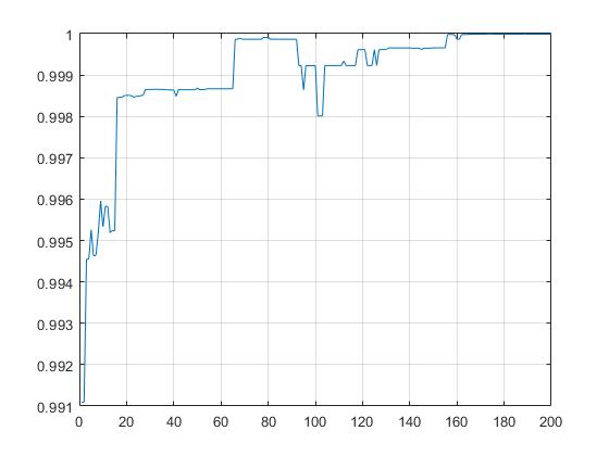
SPMEP fitness curve (EP and CEP fall into local optimization)
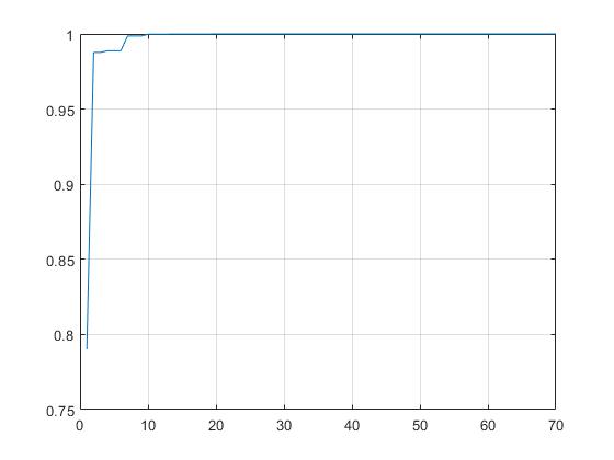
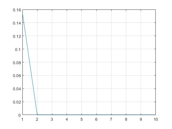 GA toolbox solution
%% GA solve
global fitall_ga;
fitall_ga = zeros(1, iter_max);
ops = optimoptions('ga', 'Generations', iter_max, 'OutputFcn', @myout);
[minx_ga, minf_ga, ~, output, population, scores]=ga(@obj_func_7x, 10, [], [], [], [], LB, UB,[],ops);
plot(1:output.generations, fitall_ga(:, 1:output.generations));
grid on;

Reference
Optimization method and its Matlab implementation