1. Stability of sorting algorithm
Stability: the stable sorting algorithm will maintain the relative order of records with equal key values. That is, if a sorting algorithm is stable, when there are two records R and S with equal key values, and R appears before S in the original list, R will also be before S in the sorted list.
When equal elements are indistinguishable, such as integers, stability is not a problem. However, suppose that the following number pairs will be sorted by their first number.
(4, 1) (3, 1) (3, 7)(5, 6)
In this case, there may be two different results. One is to maintain the relative order of records with equal key values, while the other does not:
(3, 1)  (3, 7)  (4, 1)  (5, 6)  (Maintenance order)
(3, 7)  (3, 1)  (4, 1)  (5, 6)  ((order changed)
Unstable sorting algorithms may change the relative order of records in equal key values, but stable sorting algorithms never do so. Unstable sorting algorithms can be specifically implemented as stable. One way to do this is to manually expand the comparison of key values, so that the comparison between two objects with the same key value in other aspects (for example, add the second standard in the above comparison: the size of the second key value) will be determined to use the items in the original data order as a same finals. However, keep in mind that this order usually involves an additional space burden.
2. Bubble sorting
Bubble Sort is a simple sort algorithm. It repeatedly traverses the sequence to be sorted, compares two elements at a time, and swaps them if they are in the wrong order. The work of traversing the sequence is repeated until there is no need to exchange, that is, the sequence has been sorted. The name of this algorithm comes from the fact that smaller elements will slowly "float" to the top of the sequence through exchange.
The bubble sorting algorithm operates as follows:
(1) Compare adjacent elements. If the first one is larger than the second (in ascending order), exchange them.
(2) Do the same for each pair of adjacent elements, from the first pair at the beginning to the last pair at the end. After this step, the last element will be the maximum number.
(3) Repeat the above steps for all elements except the last one.
(4) Continue to repeat the above steps for fewer and fewer elements at a time until no pair of numbers need to be compared.
2.1 analysis of bubble sorting
Diagram of exchange process (for the first time):

n-1 bubbling processes are required, and the corresponding comparison times are shown in the figure below:
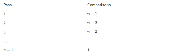
Summary: key points for bubble sorting:
(1) When sorting n data, bubble (n-1) round is required when the optimal time complexity is not considered.
(2) When bubbling in each round, it will bubble (n-1-i) times with the increase of the number of specific rounds. i: Indicates the i-th round of bubbling.
2.2 code implementation of bubble sorting
def bubble_sort(alist):
    n =len(alist)
    for i in range(n-1):
        count = 0	#The counts here prepare for the time complexity of the optimal algorithm
        for j in range(n-1-i):
            if alist[j] > alist[j+1]:
                alist[j],alist[j+1]=alist[j+1],alist[j]
                count += 1
        if 0 == count:
            print("There is no exchange in the bubble sorting process, and the time complexity of the algorithm is the best O(n)")
            break
2.3 time complexity
(1) Optimal time complexity: O(n) (indicates that no elements can be exchanged after traversing once, and the sorting ends.)
(2) Worst time complexity: O(n^2)
(3) Stability: stable
3. Select Sorting
Selection sort is a simple and intuitive sorting algorithm. Its working principle is as follows. First, find the smallest (large) element in the unordered sequence and store it at the beginning of the sorted sequence. Then, continue to find the smallest (large) element from the remaining unordered elements, and then put it at the end of the sorted sequence. And so on until all elements are sorted.
The main advantage of selective sorting is related to data movement. If an element is in the correct final position, it will not be moved. Select sort to exchange a pair of elements each time, and at least one of them will be moved to its final position. Therefore, sort the table of n elements and exchange at most n-1 times in total. Among all the sorting methods that completely rely on exchange to move elements, selective sorting is a very good one.
3.1 select sorting analysis
Sorting process:

Summary: select key points for sorting:
(1) To sort n data, select (n-1) rounds.
(2) During each round of selection, each data shall be compared with all the remaining data (i+1,n). i represents the i-round selection.
3.2 Select Sorting code implementation
def select_sort(alist):
    n = len(alist)
    min_index = 0
    for i in range(n - 1):	#N data for n-1 round operation
        for j in range(i + 1, n):	#Each data should be compared with all the remaining data
            if alist[min_index] > alist[j]:
                min_index = j	#Reset minimum index
                alist[min_index], alist[j] = alist[j], alist[min_index]
        alist[min_index], alist[i] = alist[i], alist[min_index]


li = [12, 2432, 3, 4654, 5, 43, 143,3]
select_sort(li)
print(li)
3.3 time complexity
(1) Optimal time complexity: O(n^2)
(2) Worst time complexity: O(n^2)
(3) Stability: unstable (considering the maximum selection of ascending order each time)
4. Insert sort
Insertion Sort (English: Insertion Sort) is a simple and intuitive sorting algorithm. Its working principle is to build an ordered sequence, scan the unordered data from back to front in the sorted sequence, find the corresponding position and insert it. In the implementation of insertion sorting, in the process of scanning from back to front, it is necessary to repeatedly move the sorted elements back step by step to provide insertion space for the latest elements.
4.1 insert sort analysis

Summary: insert sorted keys:
(1) N data are sorted and (n-1) rounds are inserted.
(2) During each round of insertion, the data to be inserted shall be compared with the ordered data arranged in front to find the appropriate insertion position.
(3) When the data to be sorted is already ordered data, each data does not move during each round of insertion, and its own position is the optimal position. At this time, the time complexity of the algorithm is O(n).
4.2 insert sorting implementation code
def insert_sort(alist):
    n=len(alist)
    for i in range(n-1):
        j = i
        while j > 0:
            if alist[j] < alist[j-1]:
                alist[j],alist[j-1]=alist[j-1],alist[j]
                j -=1
            else:		#The code is optimized here. When the sequence to be sorted is already an ordered sequence, no comparison insertion is performed.
                break
4.3 time complexity
(1) Optimal time complexity: O(n) (in ascending order, the sequence is already in ascending order)
(2) Worst time complexity: O(n2)
(3) Stability: stable
5. Hill sort
Shell sort is a kind of insert sort. Also known as reduced incremental sorting, it is a more efficient improved version of the direct insertion sorting algorithm. Hill sorting is an unstable sorting algorithm. This method is named after DL. Shell in 1959. Hill sort is to group records by certain increment of subscript, and sort each group by direct insertion sort algorithm; As the increment decreases, each group contains more and more keywords. When the increment decreases to 1, the whole file is just divided into one group, and the algorithm terminates.
5.1 Hill sorting process
The basic idea of hill sorting is to list the array in a table and insert the columns respectively. Repeat this process, but use longer columns each time (longer step and fewer columns). Finally, the whole table has only one column. The purpose of converting arrays to tables is to better understand the algorithm. The algorithm itself still uses arrays for sorting.
For example, suppose there is such a set of numbers [13 14 94 33 82 25 59 94 65 23 45 27 73 25 39 10], if we start sorting with a step of 5, we can better describe the algorithm by putting this list in a table with 5 columns, so that they should look like this (the vertical elements are composed of steps):
13 14 94 33 82
25 59 94 65 23
45 27 73 25 39
10
Sort each column:
10 14 73 25 23
13 27 94 33 39
25 59 94 65 82
45
When the above four lines of numbers are connected together in sequence, we get: [10 14 73 25 23 13 27 94 33 39 25 59 94 65 82 45]. At this time, 10 has moved to the correct position, and then sort in steps of 3:
10 14 73
25 23 13
27 94 33
39 25 59
94 65 82
45
After sorting, it becomes:
10 14 13
25 23 33
27 25 59
39 65 73
45 94 82
94
Finally, sort in 1 step (this is a simple insertion sort)
5.2 analysis of Hill ranking

5.3 implementation of hill sorting code
def shell_sort(alist):
    n=len(alist)
    gap = n//2
    while gap > 0:
        for i in range(gap,n):
            j = i
            while j> 0:
                if alist[j] < alist[j-gap]:
                    alist[j],alist[j-gap]=alist[j-gap],alist[j]
                    j -=gap
                else:
                    break
        gap = gap//2
5.4 time complexity
(1) Optimal time complexity: it varies according to the step sequence
(2) Worst time complexity: O(n2)
(3) Stability: unstable
6. Quick sort
Quicksort (English: quicksort), also known as partition exchange sort, divides the data to be sorted into two independent parts through one-time sorting. All the data in one part is smaller than all the data in the other part, and then quickly sort the two parts of data respectively according to this method. The whole sorting process can be recursive, So that the whole data becomes an ordered sequence.
The steps are:
(1) Picking out an element from a sequence is called a "pivot".
(2) Reorder the sequence. All elements smaller than the benchmark value are placed in front of the benchmark, and all elements larger than the benchmark value are placed behind the benchmark (the same number can be on either side). After the partition, the benchmark is in the middle of the sequence. This is called a partition operation.
Recursively sorts subsequences that are smaller than the reference value element and subsequences that are larger than the reference value element.
(3) The bottom case of recursion is that the size of the sequence is zero or one, that is, it has always been sorted. Although it recurses all the time, the algorithm will always end, because in each iteration, it will put at least one element to its last position.
6.1 analysis of quick sort

6.2 implementation of quick sort code
(1) Implementation method I
def quick_sort(alist, start, end):
    """Quick sort"""
    # Quick sort exit condition
    if start >= end:
        return
    # Set the starting element as the base element to find the position
    mid = alist[start]
    # low is the cursor that the sequence moves from left to right
    low = start
    # high is the cursor that moves the sequence from right to left
    high = end
    while low < high:
        # The low and high cursors do not coincide. If the element pointed by the high cursor is larger than the mid, the high cursor moves to the left
        while low < high and alist[high] >= mid:
            high -= 1
        # Place the element pointed by the high cursor in the low position
        alist[low] = alist[high]
        # The low and high cursors do not coincide. If the element pointed by the low cursor is larger than the mid, the low cursor moves to the right
        while low < high and alist[low] < mid:
            low += 1
        # Put the element pointed by the low cursor in the high position
        alist[high] = alist[low]
    # After exiting the loop, low coincides with high, and the indicated position is the correct position of the datum element
    # Place the base element at this position in the original list
    alist[low] = mid
    # Quick sort the subsequence to the left of the base element
    quick_sort(alist, start, low - 1)
    # Quick sort the subsequence to the right of the base element
    quick_sort(alist, low + 1, end)


if __name__ == "__main__":
    li = [54, 26, 93, 17, 77, 31, 44, 55, 20, 87, 90]
    print(li)
    quick_sort(li, 0, len(li) - 1)
    print(li)

Execution results:
	[54, 26, 93, 17, 77, 31, 44, 55, 20, 87, 90]
	[17, 20, 26, 31, 44, 54, 55, 77, 87, 90, 93]
(2) Implementation method 2
def quick_sort(alist):
    if len(alist) < 2:
        return alist
    mid = alist[len(alist) // 2]
    left, right = [], []
    alist.remove(mid)
    for i in range(len(alist)):
        if alist[i] >= mid:
            right.append(alist[i])
        else:
            left.append(alist[i])
    return quick_sort(left) + [mid] + quick_sort(right)


if __name__ == "__main__":
    li = [54, 26, 93, 17, 77, 31, 44, 55, 20, 87, 90]
    print(li)
    # quick_sort(li, 0, len(li) - 1)
    li_sort = quick_sort(li)
    print(li_sort)


Execution results:
	[54, 26, 93, 17, 77, 31, 44, 55, 20, 87, 90]
	[17, 20, 26, 31, 44, 54, 55, 77, 87, 90, 93]
6.3 time complexity
(1) Optimal time complexity: O(nlogn)
(2) Worst time complexity: O(n^2)
(3) Stability: unstable
The description of the average O(nlogn) time required for quick sorting from the beginning is not obvious. However, it is not difficult to observe the partition operation. The elements of the array will be visited once in each cycle, using O(n) time. In the version using concatenation, this operation is also O(n).
In the best case, each time we run the partition, we divide a sequence into two nearly equal segments. This means that each recursive call handles a half size sequence. Therefore, we only need to make log n nested calls before reaching the sequence with size one. This means that the depth of the call tree is O(log n). However, in two program calls of the same hierarchy, the same part of the original sequence will not be processed; Therefore, each hierarchy of program calls only needs O(n) time in total (each call has some common additional cost, but because there are only O(n) calls in each hierarchy, these are summarized in the O(n) coefficient). The result is that this algorithm only needs O(nlogn) time.
7. Merge and sort
Merge sort is a very typical application of divide and conquer. The idea of merge sort is to recursively decompose the array, and then merge the array.
After the array is decomposed to the minimum, then two ordered arrays are merged. The basic idea is to compare the front numbers of the two arrays. Whoever is small will take the first one, and the corresponding pointer will move back one bit after taking it. Then compare until one array is empty, and finally copy the rest of the other array.
7.1 code implementation of merging and sorting
def merge_sort(alist):
	"""Merge sort"""
	n = len(alist)
	# After the data in the list is decomposed into a single number, it is returned for comparison
	if n <= 1:
		return alist
	mid = n // 2
	# Decompose the list one by one
	left_list = merge_sort(alist[:mid])
	right_list = merge_sort(alist[mid:])

	# Set the left and right cursors to compare the left in this recursion_ list,right_list two sub lists
	left_pointer = 0
	right_pointer = 0
	# Set the sub list returned after this recursion
	result = []
	# By moving the left and right cursors to compare the two sublist elements, the two sublists are merged into a higher-level ordered sublist
	while left_pointer < len(left_list) and right_pointer < len(right_list):
		if left_list[left_pointer] < right_list[right_pointer]:
			result.append(left_list[left_pointer])
			left_pointer += 1
		else:
			result.append(right_list[right_pointer])
			right_pointer += 1
	# Move left_list,right_ The remaining elements in the list are appended (the original list element is
	# If the number of left_list s is odd / even, and the number of right_list s is even
	# In the case of number of cycles / periods, there will be residual yuan in the left_list or right_list after the cycle ends
	# Element, and then merge the remaining elements with result)
	result += (left_list[left_pointer:])
	result += (right_list[right_pointer:])
	return result

list1 = [11,45,3,1,5,67,890,12,34,45,66,45]
print(list1)
list1_merge = merge_sort(list1)
print(list1_merge)

Execution results:
	[11, 45, 3, 1, 5, 67, 890, 12, 34, 45, 66, 45]
	[1, 3, 5, 11, 12, 34, 45, 45, 45, 66, 67, 890]
7.2 time complexity
(1) Optimal time complexity: O(nlogn)
(2) Worst time complexity: O(nlogn)
(3) Stability: stable
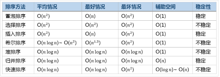
8. Efficiency comparison of common sorting algorithms