R language survival analysis: analysis of lymphoma patients with time-varying competitive risk model

Posted by prometheuzz on Thu, 17 Feb 2022 18:47:12 +0100

Original link: http://tecdat.cn/?p=22422

In this paper, we describe a flexible competitive risk regression model. The regression model is designated as the transition probability, that is, the cumulative incidence in the competitive risk setting. The model includes the model of Fine and Gray (1999) as a special case. This can be used to test the fitting degree of the proportion hypothesis of sub distribution risk (Scheike and Zhang, 2008). Confidence intervals can also be constructed for the predicted cumulative incidence rate curves. We applied these methods to Pintilie's (2007) follicular cell lymphoma data, where the competitive risk is disease recurrence and death without recurrence.

Working example: follicular cell lymphoma study

We considered Pintilie's (2007) follicular cell lymphoma data. The data set consisted of 541 patients with follicular cell lymphoma (I or II) in the early stage of the disease and received radiotherapy alone (chemotherapy = 0) or a combination of radiotherapy and chemotherapy (chemotherapy = 1). Disease recurrence or unresponsiveness and remission death are two competing risks. The patient's age (age: mean = 57, sd=14) and hemoglobin level (hgb: mean = 138, sd=15) were also recorded. The median follow-up time was 5.5 years. First, we read the data, calculate the cause of death index and encode the covariates.

R> table(cause)
cause
0 1 2
193 272 76
R> stage <- as.numeric(clinstg == 2)
R> chemo <- as.numeric(ch == "Y")
R> times1 <- sort(unique(time[cause == 1]))

There were 272 (no treatment response or recurrence) disease-related events, 76 competitive risk events (recurrence free deaths) and 193 deleted individuals. The event time is represented by dftime. The variable times1 gives the time of the event with the reason "1". We first estimated the nonparametric cumulative incidence rate curve.

We specify the event time and delete the variable cause == 0. The regression model contains only one intercept term (+ 1). The cause variable gives the reasons associated with different events. cause= 1 specifies that we consider events of type 1. The time of calculation / estimation can be given by the parameter times = times1.

Figure 1 (a) shows the cumulative incidence curve of the estimated two causes. In Figure 1 (b), we construct 95% confidence intervals (dashed lines) and 95% confidence bands.

risk(Surv(dftime, cause == 0) ~ + 1, 
causeS = 1, n.sim = 5000, cens.code = 0, model = "additive")

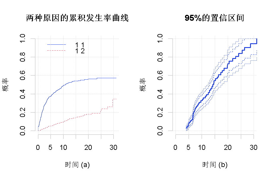
Figure 1

R> fit <- cum(time, cause, group)
R> plot(fit)

Both the sub distribution hazard method and the direct binomial model method are pruning weighting techniques based on inverse probability. The key to apply this weight is that the estimation of the weight reduction can not be biased, otherwise the estimation of cumulative incidence rate may be biased.

In this example, we found that the deletion distribution obviously depends on the covariates hemoglobin, stage and chemotherapy, and can be well described by Cox's regression model. The fitting of Cox model is verified by cumulative residuals. See Martinussen and Scheike (2006) for further details. Therefore, using simple Kaplan Meier estimation for the elimination weight may lead to serious deviation estimation. Therefore, we added cENS. Net to the call Model = "Cox", which uses all covariates of the competitive risk model in the Cox model as the elimination weight. In general, the regression model of inverse probability pruning weight can be used to improve efficiency (Scheike et al., 2008).

Now let's fit the model

We first fit a general scale model that allows all covariates to have time-varying effects. In the following call, only the covariate x in model (6) is defined. The covariant z in model (6) is specified by a const operator.

summary(outf)
OUTPUT:
Competing risks Model
Test for nonparametric terms
Test for non-significant effects
Supremum-test of significance p-value H_0: B(t)=0
(Intercept) 3.29 0.0150
stage 5.08 0.0000
age 4.12 0.0002
chemo 2.79 0.0558
hgb 1.16 0.8890
Test for time invariant effects
Kolmogorov-Smirnov test p-value H_0:constant effect
(Intercept) 8.6200 0.0100
stage 1.0400 0.0682
age 0.0900 0.0068
chemo 1.7200 0.0004
hgb 0.0127 0.5040
Cramer von Mises test p-value H_0:constant effect
(Intercept) 3.69e+01 0.0170
stage 2.52e+00 0.0010
age 4.26e-03 0.0014
chemo 1.50e+00 0.0900
hgb 2.64e-04 0.4220

The significance test based on nonparametric test showed that in the nonparametric model, stage and age were significant, chemotherapy was significant (p = 0.056), and hemoglobin was not significant (p = 0.889).

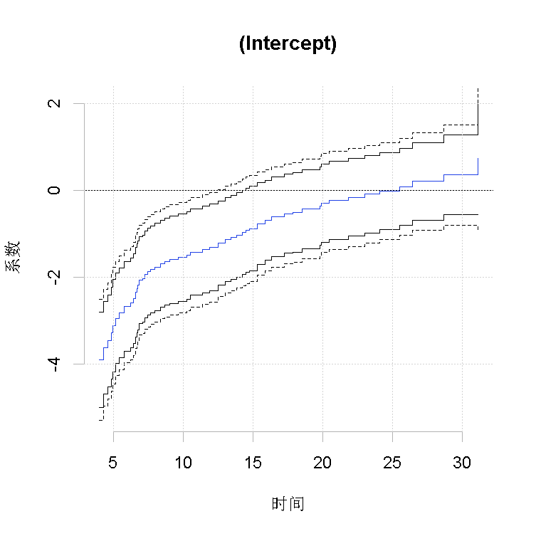
Figure 2

Plot estimated regression coefficients α j (t) and its 95% confidence band, and draw the observation test process of constant effect and the simulation test process under null value respectively.

R> plot(outf, score = 1)

Figure 2 shows that these effects do not change with time, and the effects are quite obvious in the early time period. 95% directional confidence interval and 95% confidence interval.

Figure 3 shows the relevant test process to determine whether the time-varying effect has significant time variability or whether H0 is acceptable: α j (t) = β j. The summary of these figures is given in the output. We see that the stage and chemotherapy are obviously time-varying, so they are inconsistent with the fine gray model. Kolmogorov Smirnov and Cramer von Mises test statistics are consistent with the two different summaries of the test process. The general conclusion is that the three variables have no proportional Cox type effect. We see that hemoglobin is well described by constants, so we consider a model in which hemoglobin has constant effect and other covariates have time-varying effect.

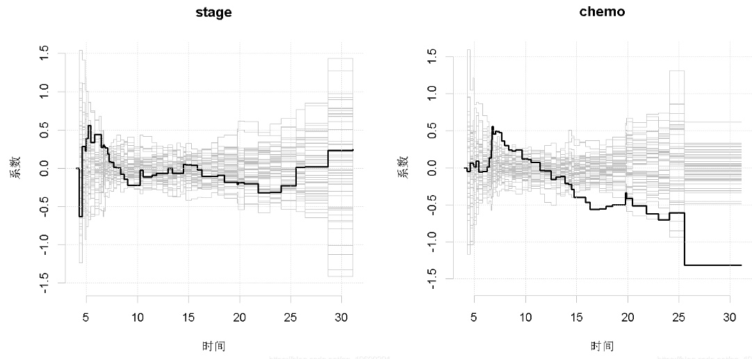
Figure 3

R> summary(outf1)
OUTPUT:
Competing risks Model
Test for nonparametric terms
Test for non-significant effects
Supremum-test of significance p-value H_0: B(t)=0
(Intercept) 5.46 0
stage 5.18 0 age 4.20 0
chemo 3.89 0
Test for time invariant effects
Kolmogorov-Smirnov test p-value H_0:constant effect
(Intercept) 10.100 0.000
stage 1.190 0.048
age 0.101 0.004
chemo 1.860 0.000
Cramer von Mises test p-value H_0:constant effect
(Intercept) 79.90000 0.000
stage 1.84000 0.006
age 0.00583 0.000
chemo 2.53000 0.000
Parametric terms :
Coef. SE Robust SE z P-val
const(hgb) 0.00195 0.00401 0.00401 0.486 0.627

Competing risks Model
Test for nonparametric terms
Test for non-significant effects
Supremum-test of significance p-value H_0: B(t)=0
(Intercept) 6.32 0
Test for time invariant effects
Kolmogorov-Smirnov test p-value H_0:constant effect
(Intercept) 1.93 0
Cramer von Mises test p-value H_0:constant effect
(Intercept) 14.3 0
Parametric terms :
Coef. SE Robust SE z P-val
const(stage) 0.45200 0.13500 0.13500 3.340 0.000838
const(age) 0.01450 0.00459 0.00459 3.150 0.001610
const(chemo) -0.37600 0.18800 0.18800 -2.000 0.045800
const(hgb) 0.00249 0.00401 0.00401 0.622 0.534000

We note that the effect of hemoglobin is almost equal to that of a more suitable model (as shown in the figure above). The estimated values of other covariates in the model may be seriously misleading, but there may be serious deviations in the estimated values of other covariates. Finally, we compare the prediction of FG model with that of semi parametric model, which describes the effect in more detail. We consider predicting two different patients as defined below by the new data allocation. Patient type I: disease stage I (stage = 0), 40 years old, without chemotherapy (chemotherapy = 0), patient type II: disease stage II (stage = 1), 60 years old, combined radiotherapy and chemotherapy (chemotherapy = 1).

R> newdata <- data.frame(stage = c(0, 1), age = c(40, 60), chemo = c(0, 1),
+ hgb = c(138, 138))
R> predict(out, newdata)

To specify the data to calculate the forecast, we can specify a newdata parameter.

The prediction based on this model may not be monotonic. We plotted predictions without point confidence intervals (se = 0) and without confidence bands (uniform = 0). The prediction in Figure 4 (a) is based on the flexible model, while the prediction in Figure 4 (b) is based on the FG model. The cumulative recurrence rate curves of type I and type II patients are represented by solid lines and dotted lines respectively. Figure 5 (a) compares the prediction results of type I patients based on flexible model and FG model. Similarly, figure 5 (b) compares the predictions for type II patients. The broken line around the two predicted values represents the confidence zone based on the flexible model.

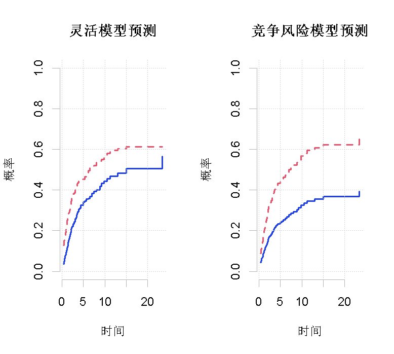
Figure 4

R> par(mfrow = c(1, 2))
R> plot(f1, se = 0, uniform = 1, col = 1, lty = 1
R> plot(fg, new = 0, se = 0, uniform = 0, col = 2, lty = 2,

The higher disease stage, higher age and combined treatment led to higher cumulative incidence rate, which was more pronounced in the early part of time (Fig. 4 (a) and Figure 2). On the other hand, chemotherapy initially increased cumulative incidence rate in time and subsequently reduced the incidence rate (Figure 4 (a) and Figure 2). Figure 5 shows that the FG model can not accurately simulate the time-varying effect. Despite these differences, in this case, the overall forecast is somewhat similar, especially when considering the uncertainty of the estimation. However, the time-varying behavior of covariates is obviously important.

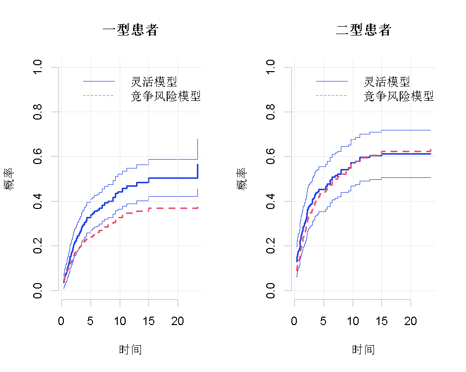
Figure 5

4. Discussion

This paper implements a flexible competition risk regression model for cumulative incidence rate curves, which can analyze in detail how covariate effect predicts cumulative incidence rate and allow time variation effect of covariates. It can check the fitting degree of simpler models and produce prediction results with confidence intervals and confidence bands, which is very useful for researchers.

Programmer Think

R language survival analysis: analysis of lymphoma patients with time-varying competitive risk model

Original link: http://tecdat.cn/?p=22422

Working example: follicular cell lymphoma study

4. Discussion

Hot Topics