preface

In NLP competition, confrontation training is a common means to improve points. This paper will introduce the scene, function, type, specific implementation and future prospect of confrontation training in detail.

Confrontation training application scenario

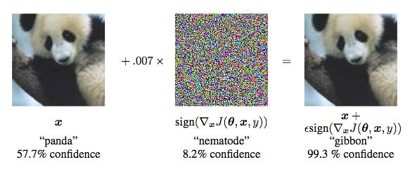
Szegedy proposed the concept of countermeasure sample in the 14 year ICLR. Confrontation samples can be used for attack and defense, and confrontation training is actually a way of defense in the "confrontation" family. Its basic principle is: build confrontation samples by adding disturbances and feed them into the model for training, so as to improve the robustness of the model when encountering confrontation samples. At the same time, it can also improve the performance and generalization ability of the model to a certain extent.

Countermeasure samples generally need to have two characteristics:

1. Compared with the original input, the added disturbance is small;
2. Can make the model wrong.

The formula of confrontation training is as follows:
min ⁡ θ E ( x , y ) ∼ D [ max ⁡ r a d v ∈ S L ( θ , x + r a d v , y ) ] \min _{\theta} \mathbb{E}_{(x, y) \sim \mathcal{D}}\left[\max _{r_{a d v} \in \mathcal{S}} L\left(\theta, x+r_{a d v}, y\right)\right] θmin​E(x,y)∼D​[radv​∈Smax​L(θ,x+radv​,y)]
The process can be divided into two steps:

1. Internal max process: find the disturbance that makes the model make the biggest mistake
2. External min process: find the parameters with the minimum overall loss

In the image field, the disturbance can be the noise on the image, but in NLP, if the disturbance is directly added to the word coding, the input will deviate from the original semantics. Because words with similar semantics in vector space are close to each other, adding a small disturbance to vector space will not cause great damage to semantics. Therefore, the current confrontation training in NLP is disturbed for embedding.

The role of confrontation training

1. Improve the robustness of the model to deal with malicious countermeasure samples.
2. As a regularization method, it can reduce overfitting and improve generalization ability.

In NLP tasks, the role of confrontation training is no longer to defend against gradient based malicious attacks, but more as a regularization method to improve the generalization ability of the model.

Specific methods of confrontation training: FGM/PGD/FreeLB

API introduction

Before introducing the specific implementation of countermeasure training, this paper first introduces the following common functions in pytoch Code:

General optimization process:

# zero the parameter gradients
optimizer.zero_grad()
# forward + backward + optimize
outputs = net(inputs)
loss = criterion(outputs, labels)
loss.backward()
optimizer.step()

Specific deployment process:

# gradient descent
weights = [0] * n
alpha = 0.0001
max_Iter = 50000
for i in range(max_Iter):
    loss = 0
    d_weights = [0] * n
    for k in range(m):
        h = dot(input[k], weights)
        d_weights = [d_weights[j] + (label[k] - h) * input[k][j] for j in range(n)] # Gradient descent optimization
        loss += (label[k] - h) * (label[k] - h) / 2 # Gradient descent optimization
    d_weights = [d_weights[k]/m for k in range(n)]
    weights = [weights[k] + alpha * d_weights[k] for k in range(n)]
    if i%10000 == 0:
        print "Iteration %d loss: %f"%(i, loss/m)
        print weights

It can be found that they are actually one-to-one correspondence:

• optimizer.zero_grad() corresponds to d_weights = [0] * n

This step initializes the gradient to zero (because the derivative of a batch's loss with respect to weight is the cumulative sum of the derivatives of all sample s' loss with respect to weight)

• outputs = net(inputs) corresponds to h = dot(input[k], weights)

This step is forward propagation to calculate the predicted value

• loss = criterion(outputs, labels) corresponding loss += (label[k] - h) * (label[k] - h) / 2

This step is to find the current specific loss value

• loss.backward() corresponds to d_weights = [d_weights[j] + (label[k] - h) * input[k][j] for j in range(n)]

This step is back propagation to find the gradient

• optimizer.step() corresponds to weights = [weights[k] + alpha * d_weights[k] for k in range(n)]

This step updates all parameters

FGSM/FGM

The idea of this method is that the disturbance along the rising direction of the gradient can bring the greatest damage to the model.

FGSM: the Sign function is used to normalize the gradient by max. Max normalization means that if the value in a dimension of the gradient is positive, it is set to 1; If negative, set to - 1; If 0, set to 0

FGM: L2 normalization is adopted. L2 normalization divides the value of each dimension of the gradient by the L2 norm of the gradient. Theoretically, L2 normalization more strictly retains the direction of the gradient, but max normalization is not necessarily the same as the direction of the original gradient.
F G S M : δ = ϵ S i g n ( g ) FGSM: \delta=\epsilon Sign(g) FGSM: δ=ϵSign(g)

F G M : δ = ϵ ( g / ∣ ∣ g 2 ∣ ∣ ) FGM: \delta = \epsilon (g/||g_2||) FGM:δ=ϵ(g/∣∣g2​∣∣)

his in g by ladder degree g = ∇ x ( L ( f θ ( X ) , y ) ) Where G is the gradient g = \ nabla x (L (f_{\ theta} (x, y)) Where G is the gradient g = ≓ x(L(f θ ​(X),y))

import torch
class FGM():
    def __init__(self, model):
        self.model = model
        self.backup = {}

    def attack(self, epsilon=1., emb_name='emb.'):
        # emb_ The parameter name should be replaced by the embedded parameter name in your model
        for name, param in self.model.named_parameters():
            if param.requires_grad and emb_name in name:
                self.backup[name] = param.data.clone()
                norm = torch.norm(param.grad)
                if norm != 0 and not torch.isnan(norm):
                    r_at = epsilon * param.grad / norm
                    param.data.add_(r_at)

    def restore(self, emb_name='emb.'):
        # emb_ The parameter name should be replaced by the embedded parameter name in your model
        for name, param in self.model.named_parameters():
            if param.requires_grad and emb_name in name: 
                assert name in self.backup
                param.data = self.backup[name]
        self.backup = {}
        

# initialization
fgm = FGM(model)
for batch_input, batch_label in data:
    # Normal training
    loss = model(batch_input, batch_label)
    loss.backward() # Back propagation to get normal grad
    # Confrontation training
    fgm.attack() # Add anti disturbance on embedding
    loss_adv = model(batch_input, batch_label)
    loss_adv.backward() # Back propagation, and accumulate the gradient of confrontation training on the basis of normal grad
    fgm.restore() # Restoring embedding parameters
    # Gradient descent, update parameters
    optimizer.step()
    model.zero_grad()

FGM/FGSM process summary

1. Normal forward propagation - get the gradient and loss values
2. Perform countermeasure training - add disturbance to the parameter value according to the current gradient; Forward propagation obtains loss and final gradient
3. Restore embedding parameters
4. Update the parameters of this iteration

According to the min max formula, confrontation training mainly completes the process of internal max. The idea of FGM/FGSM is to find the optimal solution along the rising direction of the gradient. However, FGM/FGSM assumes that the loss function is linear or locally linear. If it is not linear, the gradient lifting direction is not necessarily the optimal direction.

PGD

In order to solve the linear hypothesis problem in FGM, PGD is iterated several times. If the disturbance exceeds the range, the disturbance will be mapped to the specified range.
X t + 1 = ∏ X + S ( X t + ϵ ( g t / ∣ ∣ g t ∣ ∣ ) ) X_{t + 1}=\prod _{X+S}(X_t + \epsilon(g_t/||g_t||)) Xt+1​=X+S∏​(Xt​+ϵ(gt​/∣∣gt​∣∣))

his in g by ladder degree g t = ∇ x t ( L ( f θ ( X t ) , y ) ) Where g is the gradient g_t=\nabla x_t(L(f_{\theta}(X_t), y)) Where g is the gradient gt = ≓ Xt (L(f θ ​(Xt​),y))

Although PGD is very effective, its efficiency is not high. After M iterations, PGD needs m*(K + 1) iterations. The code is shown as follows:

import torch
class PGD():
    def __init__(self, model):
        self.model = model
        self.emb_backup = {}
        self.grad_backup = {}

    def attack(self, epsilon=1., alpha=0.3, emb_name='emb.', is_first_attack=False):
        # emb_ The parameter name should be replaced by the embedded parameter name in your model
        for name, param in self.model.named_parameters():
            if param.requires_grad and emb_name in name:
                if is_first_attack:
                    self.emb_backup[name] = param.data.clone()
                norm = torch.norm(param.grad)
                if norm != 0 and not torch.isnan(norm):
                    r_at = alpha * param.grad / norm
                    param.data.add_(r_at)
                    param.data = self.project(name, param.data, epsilon)

    def restore(self, emb_name='emb.'):
        # emb_ The parameter name should be replaced by the embedded parameter name in your model
        for name, param in self.model.named_parameters():
            if param.requires_grad and emb_name in name: 
                assert name in self.emb_backup
                param.data = self.emb_backup[name]
        self.emb_backup = {}

    def project(self, param_name, param_data, epsilon):
        r = param_data - self.emb_backup[param_name]
        if torch.norm(r) > epsilon:
            r = epsilon * r / torch.norm(r)
        return self.emb_backup[param_name] + r

    def backup_grad(self):
        for name, param in self.model.named_parameters():
            if param.requires_grad:
                self.grad_backup[name] = param.grad.clone()

    def restore_grad(self):
        for name, param in self.model.named_parameters():
            if param.requires_grad:
                param.grad = self.grad_backup[name]
                
pgd = PGD(model)
K = 3
for batch_input, batch_label in data:
    # Normal training
    loss = model(batch_input, batch_label)
    loss.backward() # Back propagation to get normal grad
    pgd.backup_grad()
    # Confrontation training
    for t in range(K):
        pgd.attack(is_first_attack=(t==0)) # Add anti disturbance on embedding, and back up param in the first attack data
        if t != K-1:
            model.zero_grad()
        else:
            pgd.restore_grad()
        loss_adv = model(batch_input, batch_label)
        loss_adv.backward() # Back propagation, and accumulate the gradient of confrontation training on the basis of normal grad
    pgd.restore() # Restoring embedding parameters
    # Gradient descent, update parameters
    optimizer.step()
    model.zero_grad()

PGD process summary

1. Normal forward propagation - get the gradient and loss values
2. Backup normal gradient
3. Perform K confrontation training
   1. If t=0, backup parameters; Gradient clearing; Forward propagation, calculate the gradient and loss value
   2. If t=K-1; Restore the gradient of step 1; Forward propagation, calculate the gradient and loss value
4. Restore the embedding parameter in 3.1
5. Update the parameters of this iteration

PGD is executed K times in order to obtain the disturbance of internal max in multiple steps - the disturbance is reflected in the parameters. The gradient returns to zero in each step, but the parameter values are accumulated: x ′ = x + ∑ t = 0 K r t x^{'}=x+\sum_{t=0}^{K} r_t X ′ = x + ∑ t=0K rt, finally according to the parameters x ′ x^{'} x 'and the forward propagation of the initial gradient calculate the loss and the final gradient. Finally, restore the initial parameters and update the parameters according to the final gradient.

FreeAT

In PGD, m times of back propagation and m * (K + 1) times of forward propagation are not efficient

FreeAT also sends back the gradient calculated by forward propagation

The comparison chart is:

(m/k) * k=m back propagation, (m/k) * k=m forward propagation

initialization r=0
 about epoch=1...N/m:
  For each x:
    For each step m:
      1.Take advantage of the previous step r，calculation x+r The gradient is obtained
      2.Update parameters according to gradient
      3.Update according to gradient r

FreeAT process summary

1. Normal forward propagation - get the gradient and loss values
2. Back up normal gradients
3. Perform K confrontation training
   1. The gradient and loss values are obtained by forward propagation
   2. Update parameters according to gradient
   3. Update disturbance according to gradient

Disadvantages: FreeLB points out that the problem with FreeAT is that each r is suboptimal to the current parameter (loss cannot be maximized), because the current r is composed of $r_{t-1} and and And \ theta_{t-1} meter count Out come of ， yes yes to Calculated for Calculated for \ theta_ Optimal of {T-1} $.

FreeLB

FreeLB believes that both FreeAT and YOPO have problems in obtaining the optimal r (inner max), so a PGD like method is proposed. However, PGD only uses the gradient of x+r output in the last step, while FreeLB takes the average value of r output gradient in each iteration, which is equivalent to treating the input as a K-fold virtual batch spliced by [X+r1, X+r2,..., X+rk]. The specific formula is:
m i n θ E ( Z , y ) − D ( 1 K ∑ t = 0 K − 1 m a x r t ∈ L t L ( f θ ( X + r t ) , y ) ) min_{\theta} E(Z,y) - D(\frac{1}{K} \sum_{t=0}^{K-1}max_{r_t \in L_t} L(f_{\theta}(X+r_t),y)) minθ​E(Z,y)−D(K1​t=0∑K−1​maxrt​∈Lt​​L(fθ​(X+rt​),y))
PGD formula is:
m i n θ E ( Z , y ) − D ( m a x ∣ ∣ r ∣ ∣ ≤ ϵ L ( f θ ( X + r t ) , y ) ) min_{\theta} E(Z,y) - D(max_{||r|| \le\epsilon} L(f_{\theta}(X+r_t),y)) minθ​E(Z,y)−D(max∣∣r∣∣≤ϵ​L(fθ​(X+rt​),y))
FreeLB differs from PGD as follows:

1. PGD is the gradient update parameter of the last disturbance after K iterations r, and FreeLB is the average gradient in K iterations
2. The disturbance range of PGD is within epsilon. Because the gradient is set to 0 in step 3 of the process, each projection will return to the circle centered on x in step 1 and the radius is epsilon, while x in FreeLB will iterate each time, so the range of r is more flexible and more likely to be close to the local optimum

Pseudo code is:

For each x:
  1.Initialization by uniform distribution r，gradient g Is 0
  For each step t=1...K:
    2.according to x+r Calculate forward and backward, cumulative gradient g
    3.to update r
  4.according to g/K Update gradient

class FreeLB(object):
    def __init__(self, adv_K, adv_lr, adv_init_mag, adv_max_norm=0., adv_norm_type='l2', base_model='bert'):
        self.adv_K = adv_K
        self.adv_lr = adv_lr
        self.adv_max_norm = adv_max_norm
        self.adv_init_mag = adv_init_mag    # Adv training initialize with what magnitude, that is, the value we use to initialize delta
        self.adv_norm_type = adv_norm_type
        self.base_model = base_model
    def attack(self, model, inputs, gradient_accumulation_steps=1):
        input_ids = inputs['input_ids']
        if isinstance(model, torch.nn.DataParallel):
            embeds_init = getattr(model.module, self.base_model).embeddings.word_embeddings(input_ids)
        else:
            embeds_init = getattr(model, self.base_model).embeddings.word_embeddings(input_ids)
        if self.adv_init_mag > 0:   # Is the first step of impact attack based on the original gradient (delta=0) or the countermeasure gradient (delta!=0)
            input_mask = inputs['attention_mask'].to(embeds_init)
            input_lengths = torch.sum(input_mask, 1)
            if self.adv_norm_type == "l2":
                delta = torch.zeros_like(embeds_init).uniform_(-1, 1) * input_mask.unsqueeze(2)
                dims = input_lengths * embeds_init.size(-1)
                mag = self.adv_init_mag / torch.sqrt(dims)
                delta = (delta * mag.view(-1, 1, 1)).detach()
            elif self.adv_norm_type == "linf":
                delta = torch.zeros_like(embeds_init).uniform_(-self.adv_init_mag, self.adv_init_mag)
                delta = delta * input_mask.unsqueeze(2)
        else:
            delta = torch.zeros_like(embeds_init)  # Disturbance initialization
        loss, logits = None, None
        for astep in range(self.adv_K):
            delta.requires_grad_()
            inputs['inputs_embeds'] = delta + embeds_init  # Cumulative primary disturbance delta
            inputs['input_ids'] = None
            outputs = model(**inputs)
            loss, logits = outputs[:2]  # model outputs are always tuple in transformers (see doc)
            loss = loss.mean()  # mean() to average on multi-gpu parallel training
            loss = loss / gradient_accumulation_steps
            loss.backward()
            delta_grad = delta.grad.clone().detach()  # Backup disturbed grad
            if self.adv_norm_type == "l2":
                denorm = torch.norm(delta_grad.view(delta_grad.size(0), -1), dim=1).view(-1, 1, 1)
                denorm = torch.clamp(denorm, min=1e-8)
                delta = (delta + self.adv_lr * delta_grad / denorm).detach()
                if self.adv_max_norm > 0:
                    delta_norm = torch.norm(delta.view(delta.size(0), -1).float(), p=2, dim=1).detach()
                    exceed_mask = (delta_norm > self.adv_max_norm).to(embeds_init)
                    reweights = (self.adv_max_norm / delta_norm * exceed_mask + (1 - exceed_mask)).view(-1, 1, 1)
                    delta = (delta * reweights).detach()
            elif self.adv_norm_type == "linf":
                denorm = torch.norm(delta_grad.view(delta_grad.size(0), -1), dim=1, p=float("inf")).view(-1, 1, 1)  # p='inf ', infinite norm, which obtains the maximum absolute value
                denorm = torch.clamp(denorm, min=1e-8)  # Similar to NP Clip to clamp the value between (min, max)
                delta = (delta + self.adv_lr * delta_grad / denorm).detach()  # Calculate the delta of this step and add it to the original delta value (gradient rise)
                if self.adv_max_norm > 0:
                    delta = torch.clamp(delta, -self.adv_max_norm, self.adv_max_norm).detach()
            else:
                raise ValueError("Norm type {} not specified.".format(self.adv_norm_type))
            if isinstance(model, torch.nn.DataParallel):  
                embeds_init = getattr(model.module, self.base_model).embeddings.word_embeddings(input_ids)
            else:
                embeds_init = getattr(model, self.base_model).embeddings.word_embeddings(input_ids)
        return loss, logits


if args.do_adv:
    inputs = {
        "input_ids": input_ids,
        "bbox": layout,
        "token_type_ids": segment_ids,
        "attention_mask": input_mask,
        "masked_lm_labels": lm_label_ids
    }
    loss, prediction_scores = freelb.attack(model, inputs)
loss.backward()
optimizer.step()
scheduler.step()
model.zero_grad()

class FreeLB():
    def __init__(self, model, args, optimizer, base_model='xlm-roberta'):
        self.args = args
        self.model = model
        self.adv_K = self.args.adv_K
        self.adv_lr = self.args.adv_lr
        self.adv_max_norm = self.args.adv_max_norm
        self.adv_init_mag = self.args.adv_init_mag  # Adv training initialize with what magnitude, that is, the value we use to initialize delta
        self.adv_norm_type = self.args.adv_norm_type
        self.base_model = base_model
        self.optimizer = optimizer

    def attack(self, model, inputs):
        args = self.args
        input_ids = inputs['input_ids']
        #Get embedding during initialization
        embeds_init = getattr(model, self.base_model).embeddings.word_embeddings(input_ids.to(args.device))

        if self.adv_init_mag > 0:   # Is the first step of impact attack based on the original gradient (delta=0) or the countermeasure gradient (delta!=0)
            input_mask = inputs['attention_mask'].to(embeds_init)
            input_lengths = torch.sum(input_mask, 1)
            if self.adv_norm_type == "l2":
                delta = torch.zeros_like(embeds_init).uniform_(-1, 1) * input_mask.unsqueeze(2)
                dims = input_lengths * embeds_init.size(-1)
                mag = self.adv_init_mag / torch.sqrt(dims)
                delta = (delta * mag.view(-1, 1, 1)).detach()
        else:
            delta = torch.zeros_like(embeds_init)  # Disturbance initialization
        # loss, logits = None, None


        for astep in range(self.adv_K):
            delta.requires_grad_()
            inputs['inputs_embeds'] = delta + embeds_init  # Cumulative primary disturbance delta
            # inputs['input_ids'] = None
            loss, _ = model(input_ids=None,
                            attention_mask=inputs["attention_mask"].to(args.device),
                             token_type_ids=inputs["token_type_ids"].to(args.device),
                             labels=inputs["sl_labels"].to(args.device),
                            inputs_embeds=inputs["inputs_embeds"].to(args.device))

            loss = loss / self.adv_K # Average gradient

            loss.backward()

            if astep == self.adv_K - 1:
                # further updates on delta
                break

            delta_grad = delta.grad.clone().detach()  # Backup disturbed grad
            if self.adv_norm_type == "l2":
                denorm = torch.norm(delta_grad.view(delta_grad.size(0), -1), dim=1).view(-1, 1, 1)
                denorm = torch.clamp(denorm, min=1e-8)
                delta = (delta + self.adv_lr * delta_grad / denorm).detach()
                if self.adv_max_norm > 0:
                    delta_norm = torch.norm(delta.view(delta.size(0), -1).float(), p=2, dim=1).detach()
                    exceed_mask = (delta_norm > self.adv_max_norm).to(embeds_init)
                    reweights = (self.adv_max_norm / delta_norm * exceed_mask + (1 - exceed_mask)).view(-1, 1, 1)
                    delta = (delta * reweights).detach()
            else:
                raise ValueError("Norm type {} not specified.".format(self.adv_norm_type))

            embeds_init = getattr(model, self.base_model).embeddings.word_embeddings(input_ids.to(args.device))
        return loss

for batch_input, batch_label in data:
    # Normal training
    loss = model(batch_input, batch_label)
    loss.backward() # Back propagation to get normal grad
    # Confrontation training
    freelb = FreeLB( model, args, optimizer, base_model)
    loss_adv = freelb.attack(model, batch_input)
    loss_adv.backward() # Back propagation, and accumulate the gradient of confrontation training on the basis of normal grad
    # Gradient descent, update parameters
    optimizer.step()
    model.zero_grad()

FreeLB process summary

1. Normal forward propagation - get the gradient and loss values
2. Back up normal gradients
3. Perform K confrontation training
   1. Forward propagation, calculate the gradient and loss value
   2. Gradient accumulation
   3. Calculate the disturbance according to the gradient
4. Restore initial embedding parameters
5. Update the parameters of this iteration

Like FreeAT, this method wants to make efficient use of both gradients. The difference is that this method does not update every time, but accumulates the parameter gradients and updates the parameters with the accumulated gradients.

General paradigm

Through the study of the above several confrontation training methods, it is not difficult to see that the purpose of confrontation training is to complete the task of internal max and find the optimal solution of the maximum disturbance. The specific performance is as follows: solving the maximum disturbance update parameters; The loss and final gradient are obtained by forward propagation according to the parameters; Restore the original parameter value; The final gradient is used to update the initial parameter value. Therefore, the general process is shown as follows:

1. Normal forward propagation-Get the gradient and loss value
2. Backup normal parameters
3. Solve the optimal value of disturbance and update the parameters
4. According to the updated parameters and the initial gradient, the final gradient is obtained by forward propagation
5. Restore original parameters
6. Update the parameters according to the initial parameters and the final gradient

Different countermeasure training methods are reflected in different ways to solve the optimal value of disturbance:

• The optimal value of FGM/FGSM is solved in one step, and the disturbance value is obtained according to the initial gradient and parameter value
• The optimal value of PGD is solved in multiple steps. In each step, the disturbance is obtained and the parameters are updated according to the parameters of the previous step, and finally the disturbance value accumulated in multiple steps is obtained
• The solution method of FreeAT optimal value is: it is divided into multiple steps as PGD, but this method is equivalent to: the disturbance value obtained according to the parameters and gradient of the previous step in each step is the final disturbance value
• The solution method of FreeLB optimal value is: it is divided into multiple steps like PGD, but when the gradient is updated at the end, the final gradient is the initial gradient plus the average value of each step gradient

Prospect of confrontation training

Virtual confrontation training

What is virtual confrontation training (VAT)?

VAT does not need label information and can be applied to unsupervised learning. The rising direction of its gradient can make the predicted output distribution deviate from the current direction, while the traditional confrontation training course is to make the model prediction deviate from the direction of label to the greatest extent. Therefore, VAT does not use real label, but "virtual" label - the prediction result of the current model.

In this section, you can view JayJay's blog: Virtual confrontation training: make the pre training model powerful again!

Extended thinking

Confrontation training and gradient punishment

This content is Su Shen's blog On confrontation training: significance, methods and thinking (with Keras Implementation) Mentioned in:

Assumptions have been made against disturbances Δ x. So we're updating θ When, consider L ( x + Δ x , y ; θ ) L(x+Δx,y;θ) L(x+ Δ x,y; θ) Expansion of:
min ⁡ θ E ( x , y ) ∼ D [ L ( x + Δ x , y ; θ ) ] ≈   min ⁡ θ E ( x , y ) ∼ D [ L ( x , y ; θ ) + ⟨ ∇ x L ( x , y ; θ ) , Δ x ⟩ ] \min_{\theta}\mathbb{E}_{(x,y)\sim\mathcal{D}}\left[L(x+\Delta x, y;\theta)\right]\\ \approx\, \min_{\theta}\mathbb{E}_{(x,y)\sim\mathcal{D}}\left[L(x, y;\theta)+\langle\nabla_x L(x, y;\theta), \Delta x\rangle\right] θmin​E(x,y)∼D​[L(x+Δx,y;θ)]≈θmin​E(x,y)∼D​[L(x,y;θ)+⟨∇x​L(x,y;θ),Δx⟩]

Corresponding θ The gradient of is:
∇ θ L ( x , y ; θ ) + ⟨ ∇ θ ∇ x L ( x , y ; θ ) , Δ x ⟩ \nabla_{\theta}L(x, y;\theta)+\langle\nabla_{\theta}\nabla_x L(x, y;\theta), \Delta x\rangle ∇θ​L(x,y;θ)+⟨∇θ​∇x​L(x,y;θ),Δx⟩

Substitute in Δ x = ϵ ∇ x L ( x , y ; θ ) \Delta x=\epsilon \nabla_x L(x, y;\theta) Δ x= ϵ ∇x​L(x,y; θ)， obtain
∇ θ L ( x , y ; θ ) + ϵ ⟨ ∇ θ ∇ x L ( x , y ; θ ) , ∇ x L ( x , y ; θ ) ⟩ =   ∇ θ ( L ( x , y ; θ ) + 1 2 ϵ ∥ ∇ x L ( x , y ; θ ) ∥ 2 ) \nabla_{\theta}L(x, y;\theta)+\epsilon\langle\nabla_{\theta}\nabla_x L(x, y;\theta), \nabla_x L(x, y;\theta)\rangle\\ =\,\nabla_{\theta}\left(L(x, y;\theta)+\frac{1}{2}\epsilon\left\Vert\nabla_x L(x, y;\theta)\right\Vert^2\right) ∇θ​L(x,y;θ)+ϵ⟨∇θ​∇x​L(x,y;θ),∇x​L(x,y;θ)⟩=∇θ​(L(x,y;θ)+21​ϵ∥∇x​L(x,y;θ)∥2)

This result indicates that the input sample is applied ϵ ∇ x L ( x , y ; θ ) \epsilon \nabla_x L(x, y;\theta) ϵ ∇x​L(x,y; θ) To some extent, it is equivalent to adding "gradient penalty" to loss
1 2 ϵ ∥ ∇ x L ( x , y ; θ ) ∥ 2 \frac{1}{2}\epsilon\left\Vert\nabla_x L(x, y;\theta)\right\Vert^2 21​ϵ∥∇x​L(x,y;θ)∥2

If the counter disturbance is ∇ x L ( x , y ; θ ) / ∥ ∇ x L ( x , y ; θ ) ∥ \nabla_x L(x, y;\theta)/\Vert \nabla_x L(x, y;\theta)\Vert ∇x​L(x,y; θ)/ ∥∇x​L(x,y; θ) ", then the corresponding gradient penalty term is ϵ ∥ ∇ x L ( x , y ; θ ) ∥ \epsilon\left\Vert\nabla_x L(x, y;\theta)\right\Vert ϵ ∥∇x​L(x,y; θ) ‖ (1 / 2 less and 2 less power).

In fact, this result is not new. It first appears in the paper <Improving the Adversarial Robustness and Interpretability of Deep Neural Networks by Regularizing their Input Gradients> Inside. It's just that this article is not easy to find, because once you search for keywords such as "Oriental Training gradient penalty", almost all the results are related to WGAN-GP.

Word vector space

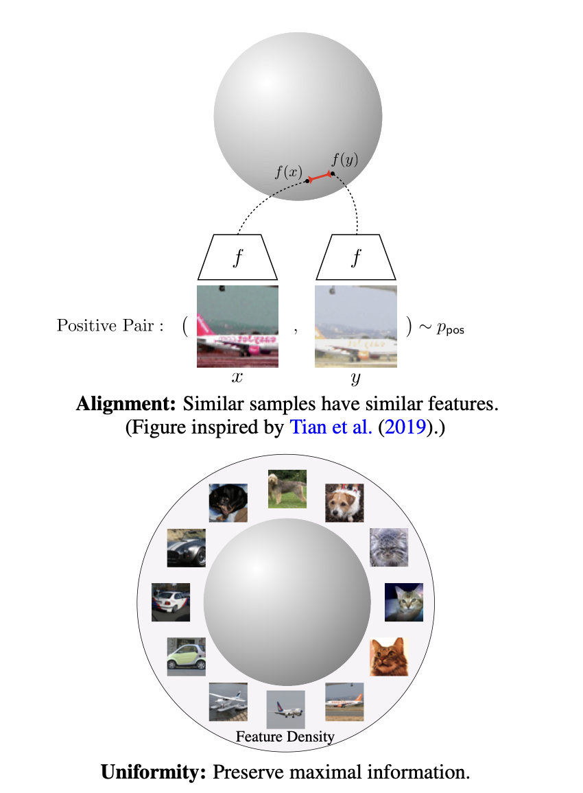
The current way of confrontation training in NLP is to add disturbance to the embedded vector space, so what is the vector space? In the research of comparative learning, it is also proposed that a good comparative learning system should have two specific characteristics:

• **Alignment: * * refers to similar examples, that is, positive examples. After mapping to the unit hypersphere, there should be close features, that is, the distance on the hypersphere is relatively close
• **Uniformity: * * means that the system should tend to retain as much information as possible in the features, which is equivalent to making the features mapped to the unit hypersphere evenly distributed on the sphere as much as possible. The more evenly distributed, the more sufficient the information retained. Even distribution means that there are differences between two, but also that each has its own unique information, which means that the information is fully retained.

In extreme cases, model collapse occurs, that is, all features are mapped to the same point:

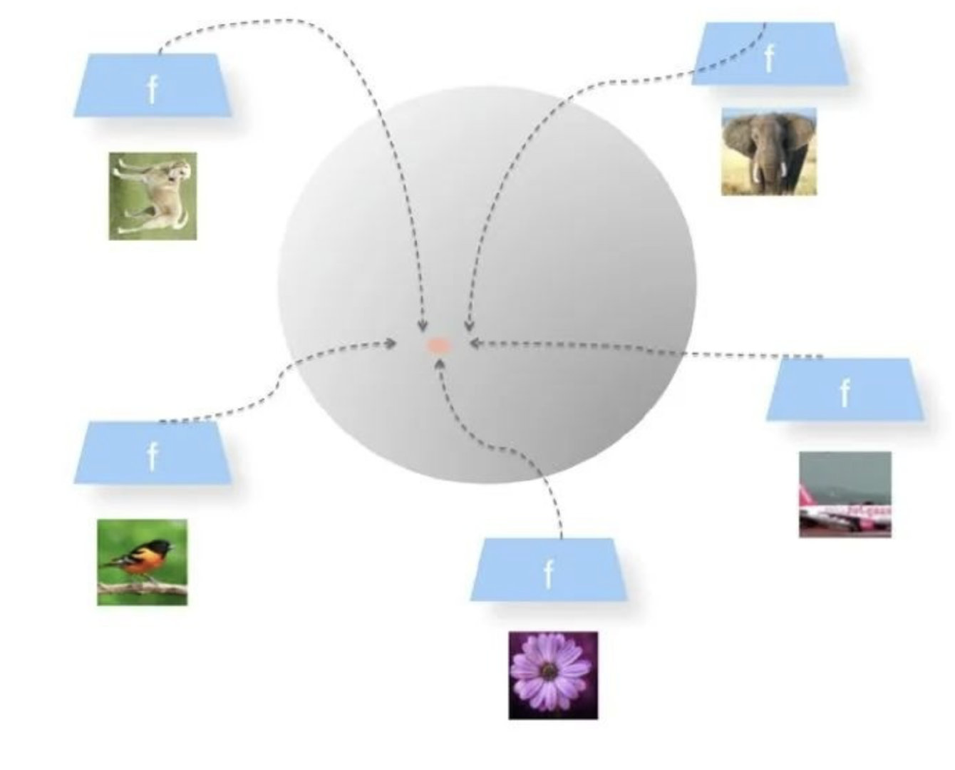
The author believes that confrontation training adds disturbance to the word vector layer, which is similar to comparative learning, realizes the similar purpose of similar examples in the vector space, and completes the task of small change in input and small change in output.