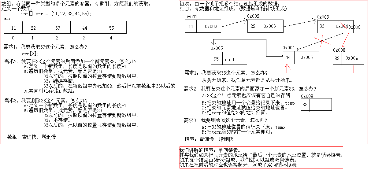
Analysis of arrays and single linked lists?

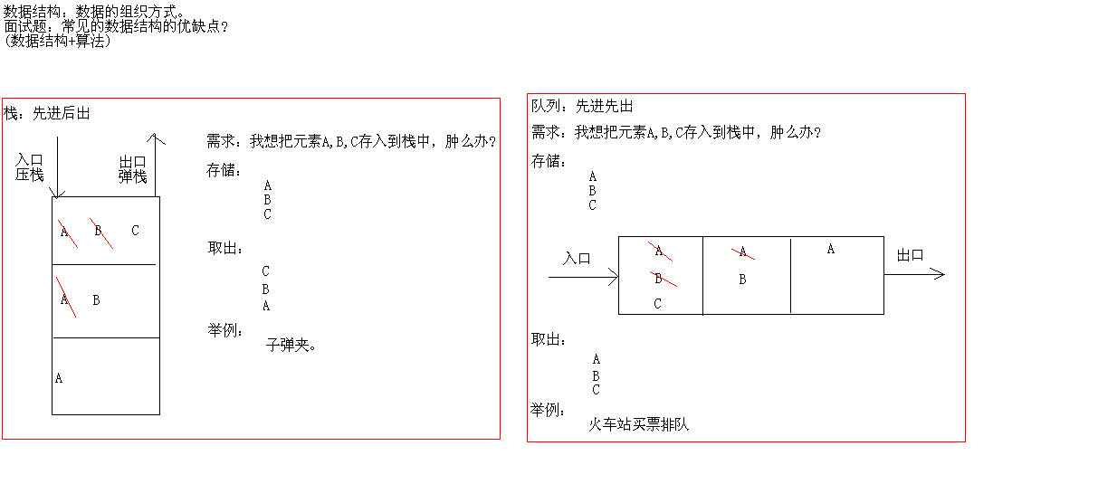
2. Analysis of stacks and teams?

I. Linear Tables

Linear table is the most common and simplest data structure. It is a finite sequence of n data elements.

There are two ways to realize linear tables. One is to use arrays to store the elements of linear tables, that is, to store the data elements of linear tables sequentially with a set of consecutive storage units. The other is to use linked lists to store elements of linear tables, that is, to store data elements of linear tables with a set of arbitrary storage units (storage units can be continuous or discontinuous).

Array is a data structure with fixed size. All operations on linear tables can be realized by array. Although the size of an array cannot be changed once it is created, when an array can no longer store new elements in a linear table, we can create a new large array to replace the current array. This allows dynamic data structures to be implemented using arrays.

• Code 1 creates a larger array to replace the current array

int[] oldArray = new int[10];
        
int[] newArray = new int[20];
        
for (int i = 0; i < oldArray.length; i++) {
    newArray[i] = oldArray[i];
}

// You can also use System.arraycopy to replicate between arrays     
// System.arraycopy(oldArray, 0, newArray, 0, oldArray.length);
        
oldArray = newArray;

• Code 2 adds element e to array position index

//oldArray represents an array of currently stored elements
//size represents the current number of elements
public void add(int index, int e) {

    if (index > size || index < 0) {
        System.out.println("Illegal location...");
    }

    //Expansion if the array is full
    if (size >= oldArray.length) {
        // Extension function reference code 1
    }

    for (int i = size - 1; i >= index; i--) {
        oldArray[i + 1] = oldArray[i];
    }

    //Move the array elementData one bit backward from all elements of the location index
    // System.arraycopy(oldArray, index, oldArray, index + 1,size - index);

    oldArray[index] = e;

    size++;
}

Above, we simply write out two typical functions of array to realize linear table. Specifically, we can refer to the source code of ArrayList collection class in Java. The advantage of linear tables implemented by arrays is that they can access or modify elements through subscripts, which is more efficient. The main disadvantage is that the cost of inserting and deleting elements is too high. For example, when an element is inserted before the first position, all elements must be moved back first. In order to improve the efficiency of adding or deleting elements at any location, a chain structure can be used to implement linear tables.

Link list is a kind of discontinuous and non-sequential storage structure on physical storage unit. The logical order of Data elements is realized by the order of pointer links in the linked list. The linked list consists of a series of nodes that do not need to be connected in memory. Each node is pointed to the next node by the Data part and the chain part Next, so when adding or deleting, only need to change the direction of the Next of the relevant node, which is very efficient.

Structure of single linked list

The following code is mainly used to show some basic operations of the linked list. It should be noted that here is mainly a single linked list as an example, without considering double linked list and circular linked list for the time being.

• Nodes in code 3 linked list

class Node<E> {

    E item;
    Node<E> next;
    
    //Constructor
    Node(E element) {
       this.item = element;
       this.next = null;
   }
}

• After code 4 defines the nodes, the head and tail nodes are usually initialized before using them.

//Head and tail nodes are empty list
Node<E> head = null;
Node<E> tail = null;

• Code 5 Create a new node from an empty list

//Create a new node and have the head point to it
head = new Node("nodedata1");

//Let the tail node also point to this node
tail = head;

• Adding a node to the code 6 list

//Create a new node and connect to the last node at the same time
tail.next = new Node("node1data2");

//Tail Node Points to New Node
tail = tail.next;

• Code 7 traverses the linked list sequentially

Node<String> current = head;
while (current != null) {
    System.out.println(current.item);
    current = current.next;
}

• Code 8 traverses the list in reverse order

static void printListRev(Node<String> head) {
//Inverse traversal list is mainly used for recursive thinking.
    if (head != null) {
        printListRev(head.next);
        System.out.println(head.item);
    }
}

• Code single list inversion

//Single list inversion is accomplished by changing the link relationship between two nodes one by one.
static Node<String> revList(Node<String> head) {

    if (head == null) {
        return null;
    }

    Node<String> nodeResult = null;

    Node<String> nodePre = null;
    Node<String> current = head;

    while (current != null) {

        Node<String> nodeNext = current.next;

        if (nodeNext == null) {
            nodeResult = current;
        }

        current.next = nodePre;
        nodePre = current;
        current = nodeNext;
    }

    return nodeResult;
}

The above code mainly shows several basic operations of the linked list. There are many operations such as getting the specified elements, removing the elements and so on. When writing these codes, we must clear up the relationship between the nodes, so that it is not easy to make mistakes.

There are other ways to realize linked list, such as cyclic single-linked list, bidirectional linked list and cyclic bidirectional linked list. Cyclic single-linked list is mainly the last node of the list pointing to the first node, which constitutes a chain as a whole. The bidirectional list is mainly composed of two pointer parts, one pointing to the precursor and one pointing to the successor. The implementation of LinkedList collection class in JDK is the bidirectional list. The ** circular bidirectional list ** is the last node pointing to the first node.

Stack and Queue

Stacks and queues are also common data structures. They are special linear tables. For stacks, elements can only be accessed, inserted and deleted at the top of the stack. For queues, elements can only be inserted from the end of the queue and accessed and deleted from the head of the queue.

Stack is a table that restricts insertion and deletion only in one location, which is the end of the table, called the top of the stack. The basic operations of the stack are push (in stack) and pop (out stack). The former is equivalent to insertion, and the latter is equivalent to deleting the last element. Stack is sometimes called LIFO(Last In First Out) table, that is, last in first out.

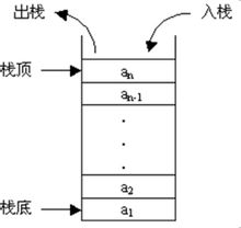
Stack model

Now let's look at a classic topic to deepen our understanding of stacks.

A classic topic about stack

The answer in the picture above is C, and the principle can be well thought over.

Because the stack is also a table, any way to implement the table can implement the stack. When we open the source code of the class Stack in JDK, we can see that it is the inheritance class Vector. Of course, Stack was a container class before Java 2, and now we can use LinkedList for all stack operations.

Queue is a special linear table. It only allows deletion at the front of the table, but insertion at the back of the table. Like stack, queue is a restricted linear table. The end of the insertion operation is called the end of the queue, and the end of the deletion operation is called the head of the queue.

Queue diagram

We can use linked lists to implement queues. The following code shows how to use LinkedList to implement queue classes.

• Code 9 simply implements the queue class

public class MyQueue<E> {

    private LinkedList<E> list = new LinkedList<>();

    // Join the team
    public void enqueue(E e) {
        list.addLast(e);
    }

    // Team out
    public E dequeue() {
        return list.removeFirst();
    }
}

Ordinary queues are a first-in-first-out data structure, and elements in priority queues are given priority. When accessing an element, the element with the highest priority is first deleted. Priority queues are still widely used in daily life. For example, emergency departments in hospitals give priority to patients, and patients with the highest priority receive treatment first. In the Java Collection Framework, the class PriorityQueue is the implementation class of the priority queue, and you can read the source code specifically.

Trees and Binary Trees

Tree structure is a very important non-linear data structure, among which tree and binary tree are most commonly used. Before introducing binary trees, let's take a brief look at the relevant content of trees.

** Tree is a hierarchical set composed of n (n >= 1) finite nodes. It has the following characteristics: each node has zero or more child nodes; nodes without parent nodes are called root nodes; each non-root node has and has only one parent node **; each child node can be divided into several disjoint subtrees except the root node.

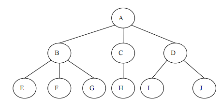
Structure of tree

• Definition

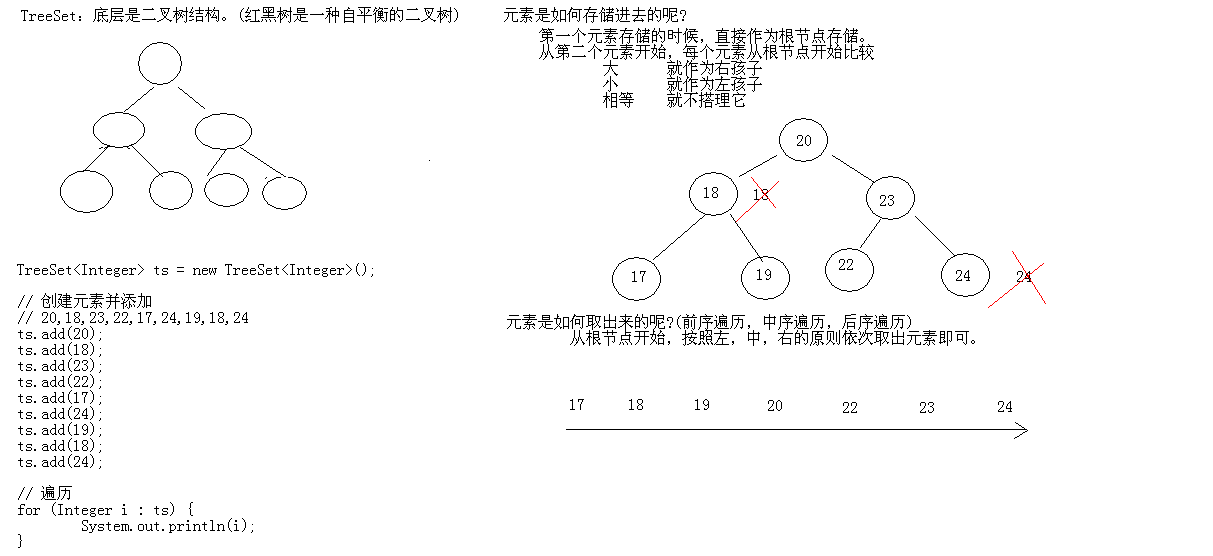
A binary tree is a tree structure with at most two subtrees per node. Usually, subtrees are called "left subtrees" and "right subtrees". Binary trees are often used to implement binary search trees and binary heaps.

• Related properties

Each node of a binary tree has at most two subtrees (there are no nodes with a degree greater than 2). The subtrees of a binary tree can be divided into left and right subtrees, and the order can not be reversed.

There are at most 2(i-1) nodes in the first layer of a binary tree, and at most 2k-1 nodes in a binary tree with a depth of K.

A binary tree with a depth of K and 2^k-1 nodes is called ** full binary tree **.

A binary tree with n nodes in depth k is called ** complete binary tree ** if and only if each of its nodes corresponds to a full binary tree with a serial number of 1 to N in depth k.

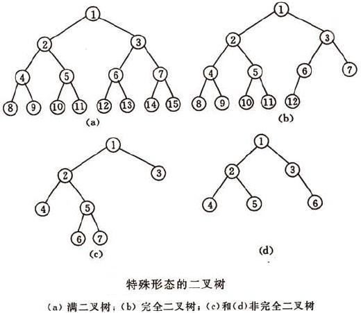
• Three ergodic methods

In some applications of binary tree, it is often required to find nodes with certain characteristics in the tree, or to deal with all nodes in the tree, which involves traversing the binary tree. The binary tree is mainly composed of three basic units: root node, left subtree and right subtree. If the order of traversal of the three parts is different, it can be divided into three categories: first traversal, middle traversal and subsequent traversal.

(1) If the binary tree is empty, the operation is empty. Otherwise, the root node is visited first, then the left subtree is traversed first, and the right subtree is traversed first. (2) If the binary tree is empty, then the operation is empty. Otherwise, the left subtree is traversed in middle order, then the root node is visited, and the right subtree is traversed in middle order. (3) If the binary tree is empty, then the operation is empty. Otherwise, the left subtree is sequentially traversed to access the root node, then the right subtree is sequentially traversed, and finally the root node is accessed.

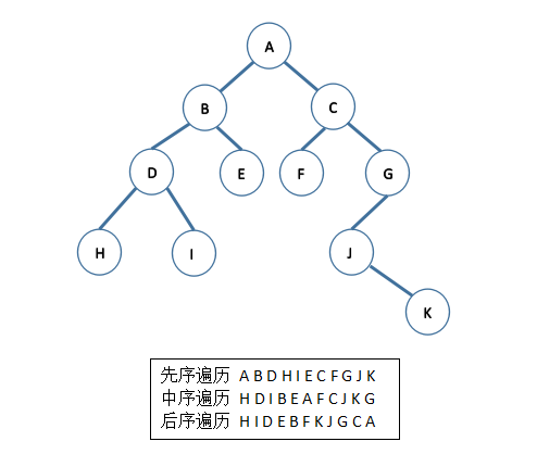
Given a binary tree, write three traversal results

• The Difference between Trees and Binary Trees

(1) Each node of the binary tree has at most two sub-nodes, while the tree is unlimited. (2) The node subtree in a binary tree is divided into left subtree and right subtree. Even if a node has only one subtree, it is necessary to indicate whether the subtree is left subtree or right subtree, that is, the binary tree is ordered. (3) A tree must never be empty, it has at least one node, and a binary tree can be empty.

Above, we mainly introduce the related concepts of binary tree. Next, we will start with the binary search tree, introduce several common types of binary tree, and implement the previous theoretical part with code.

• Definition

A binary search tree is a binary sort tree, also known as a binary search tree. A binary search tree is either an empty tree or a binary tree with the following properties: (1) if the left subtree is not empty, the values of all nodes in the left subtree are less than those of its root node; (2) if the right subtree is not empty, the values of all nodes in the right subtree are larger than those of its root node; (3) the left subtree and the right subtree are also two, respectively. Fork sort tree; (4) No nodes with equal keys.

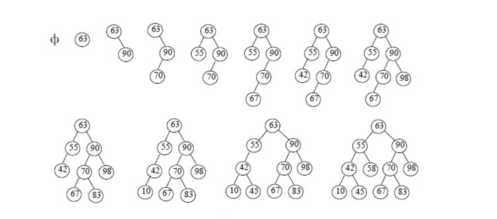
Typical Binary Search Tree Construction Process

• performance analysis

For binary lookup trees, when the given values are the same but the order is different, the shape of the binary lookup tree is different. Let's look at an example.

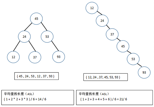
ASL of different morphologically balanced binary trees is different

It can be seen that the average search length of a binary search tree with n nodes is related to the shape of the tree. In the worst case, when keywords are inserted sequentially, the binary search tree is transformed into a single branch tree with a depth of n, and its average search length (n+1)/2 (the same as the sequential search). The best case is that the shape of the binary search tree is the same as the decision tree of the half-search, and its average search length is proportional to log2(n). O n average, the average search length and logn of the binary search tree are equal in magnitude, so in order to achieve better performance, it is usually necessary to "balance" the process of building the binary search tree. Then we will introduce the balanced binary tree and red-black tree, which can make the height of the search tree O (log (n).

• Node of Code 10 Binary Tree

class TreeNode<E> {

    E element;
    TreeNode<E> left;
    TreeNode<E> right;

    public TreeNode(E e) {
        element = e;
    }
}

The three traversals of binary search tree can be realized directly by recursive method.

• Code 12 precedence traversal

protected void preorder(TreeNode<E> root) {

    if (root == null)
        return;

    System.out.println(root.element + " ");

    preorder(root.left);

    preorder(root.right);
}

• Ordered traversal in code 13

protected void inorder(TreeNode<E> root) {

    if (root == null)
        return;

    inorder(root.left);

    System.out.println(root.element + " ");

    inorder(root.right);
}

• Post-order traversal of code 14

protected void postorder(TreeNode<E> root) {

    if (root == null)
        return;

    postorder(root.left);

    postorder(root.right);

    System.out.println(root.element + " ");
}

• A Simple Implementation of Code 15 Binary Search Tree

/**
 * @author JackalTsc
 */
public class MyBinSearchTree<E extends Comparable<E>> {

    // root
    private TreeNode<E> root;

    // Default constructor
    public MyBinSearchTree() {
    }

    // Search for Binary Search Tree
    public boolean search(E e) {

        TreeNode<E> current = root;

        while (current != null) {

            if (e.compareTo(current.element) < 0) {
                current = current.left;
            } else if (e.compareTo(current.element) > 0) {
                current = current.right;
            } else {
                return true;
            }
        }

        return false;
    }

    // Insertion of Binary Search Tree
    public boolean insert(E e) {

        // If the element previously inserted into an empty binary tree is the root node
        if (root == null) {
            root = createNewNode(e);
        } else {
            // Otherwise, traverse from the root node until the appropriate parent node is found
            TreeNode<E> parent = null;
            TreeNode<E> current = root;
            while (current != null) {
                if (e.compareTo(current.element) < 0) {
                    parent = current;
                    current = current.left;
                } else if (e.compareTo(current.element) > 0) {
                    parent = current;
                    current = current.right;
                } else {
                    return false;
                }
            }
            // insert
            if (e.compareTo(parent.element) < 0) {
                parent.left = createNewNode(e);
            } else {
                parent.right = createNewNode(e);
            }
        }
        return true;
    }

    // Create new nodes
    protected TreeNode<E> createNewNode(E e) {
        return new TreeNode(e);
    }

}

// Nodes of Binary Tree
class TreeNode<E extends Comparable<E>> {

    E element;
    TreeNode<E> left;
    TreeNode<E> right;

    public TreeNode(E e) {
        element = e;
    }
}

The above code 15 mainly shows a simple binary search tree implemented by ourselves, including several common operations, of course, more operations still need to be completed by ourselves. Because the operation of deleting nodes in the binary lookup tree is complex, I will introduce it in detail below.

• Analysis of Deleted Nodes in Binary Search Tree

To delete an element from the binary lookup tree, you first need to locate the node containing the element and its parent node. Assuming that current points to the node containing the element in the binary lookup tree and parent points to the parent node of the current node, the current node may be either the left child of the parent node or the right child of the parent node. Two situations need to be considered here:

1. The current node has no left child, so it only needs to connect the right child of the current node and the patent node.
2. The current node has a left child, assuming that rightMost points to the node that contains the largest element in the left subtree of the current node, and parentOfRightMost points to the parent of the rightMost node. Then the element values in the current node are replaced by the element values in the rightMost node, the parentOfRightMost node is connected with the left child of the rightMost node, and the rightMost node is deleted.

    // Binary Search Tree Delete Nodes
    public boolean delete(E e) {

        TreeNode<E> parent = null;
        TreeNode<E> current = root;

        // Find the location of the node to delete
        while (current != null) {
            if (e.compareTo(current.element) < 0) {
                parent = current;
                current = current.left;
            } else if (e.compareTo(current.element) > 0) {
                parent = current;
                current = current.right;
            } else {
                break;
            }
        }

        // No node to delete was found
        if (current == null) {
            return false;
        }

        // Consider the first case.
        if (current.left == null) {
            if (parent == null) {
                root = current.right;
            } else {
                if (e.compareTo(parent.element) < 0) {
                    parent.left = current.right;
                } else {
                    parent.right = current.right;
                }
            }
        } else { // Consider the second scenario
            TreeNode<E> parentOfRightMost = current;
            TreeNode<E> rightMost = current.left;
            // Find the largest element node in the left subtree
            while (rightMost.right != null) {
                parentOfRightMost = rightMost;
                rightMost = rightMost.right;
            }

            // replace
            current.element = rightMost.element;

            // parentOfRightMost is connected to the left child of rightMost
            if (parentOfRightMost.right == rightMost) {
                parentOfRightMost.right = rightMost.left;
            } else {
                parentOfRightMost.left = rightMost.left;
            }
        }

        return true;
    }

Balanced binary tree, also known as AVL tree, is either an empty tree or a binary tree with the following properties: its left and right subtrees are balanced binary trees, and the absolute value of the difference between the depth of left subtree and right subtree is not more than 1.

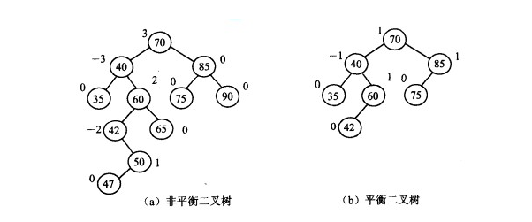
balanced binary tree

AVL tree is the first self-balanced binary search tree algorithm invented. In AVL, the maximum height difference between the two son subtrees of any node is 1, so it is also called the height balance tree. The maximum depth of the AVL tree with n nodes is about 1.44 log2n. Finding, inserting and deleting are O (log n) in average and worst case. Adding and deleting may require rebalancing the tree through one or more tree rotations.

Red-black tree is a kind of balanced binary tree, which guarantees that the event complexity of basic dynamic set operation is O(log n) in the worst case. The differences between red-black tree and balanced binary tree are as follows: (1) Red-black tree abandons the pursuit of complete balance and seeks roughly balance. Under the condition that the time complexity of the balanced binary tree is not much different from that of the balanced binary tree, the balance can be achieved by only three rotations per insertion, and the realization is simpler. (2) Equilibrium binary tree pursues absolute equilibrium with harsh conditions, which makes it difficult to realize. The number of rotations required after each insertion of new nodes cannot be predicted.