1. Introduction of Apriori correlation analysis
This part can be seen in my last blog post, which mainly introduces the principle of correlation analysis.
Link: Relevance analysis of python machine learning (Apriori).
2. Case background and analysis process
There are many kinds of modern goods, and customers often struggle with what to buy. Especially for customers with selection difficulties, it is even more difficult to choose goods. Complicated shopping often brings customers a tired shopping experience. For some commodities, such as bread and milk, potato chips and coke, customers often buy things at the same time. When these things are very far away, they will reduce customers' desire to buy. Therefore, in order to obtain the maximum sales profit, we need to know what kind of goods to sell, what kind of promotion means to use, how to place the goods on the shelf and understand customers' purchase habits and preferences, which are particularly important for sellers.
Analysis purpose:
- Construct the Apriori model of commodities and analyze the correlation between commodities.
- The sales strategy is given according to the model results.
The specific steps are as follows:
- View the form of the original data.
- Preprocess the original data and convert the data form to meet the requirements of Apriori correlation analysis.
- Establish Apriori model and adjust super parameters.
- Analyze the model results. Provide sales advice.
3. Preliminary data processing
We should have a general understanding of the data of this case. There are 9835 shopping basket data and two tables in this case. It mainly includes three attributes:
| Table name | Attribute value | describe |
|---|---|---|
| Goods Order | id | The number of the category to which the commodity belongs |
| Goods | Specific commodity name | |
| Goods Types | Goods | Specific commodity name |
| Type | Commodity category |
#This file is the main file of Apriori model
import pandas as pd
file_path=open("....Fill in the file path here//GoodsOrder.csv")
data=pd.read_csv(file_path)
data.info()
des=pd.DataFrame(data.describe()).T
print(des)#View information description
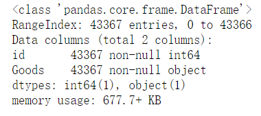
There are 43367 observed values in total, and there is no missing value. The maximum id is 9835, indicating that there are 9835 shopping basket information in total.

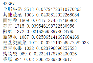
View the proportion of sales volume:
#Proportion of sales volume
data_nums = data.shape[0]
for idnex, row in sorted[:10].iterrows():#iterrows is pd's row index and data equivalent to enumerate pd by number of times
    print(row['Goods'],row['id'],row['id']/data_nums)
4. Further analysis of commodities
In step 3, we analyzed some specific commodities. Such classification has some difficulties in the implementation of follow-up decisions. We should connect these specific commodities with their own categories. Through the data in the Good Types table, we find out the category of the corresponding commodity, which is equivalent to the association in the database.
#Sales volume and proportion of various categories of goods
import pandas as pd
inputfile1 =open("C://Users / / administrator / / desktop / / Python code / / Python data analysis and mining (2nd Edition) source data and code / / Python data analysis and mining (2nd Edition) source data and code - chapters / / Chapter8 / / demo / / data / / goodorder csv")
inputfile2 =open("C://Users / / administrator / / desktop / / Python code / / Python data analysis and mining (2nd Edition) source data and code / / Python data analysis and mining (2nd Edition) source data and code - chapters / / Chapter8 / / demo / / data / / goodstypes csv")
data = pd.read_csv(inputfile1)
types = pd.read_csv(inputfile2)  # read in data

group = data.groupby(['Goods']).count().reset_index()
sort = group.sort_values('id',ascending = False).reset_index()
data_nums = data.shape[0]  # total
#print(sort)
del sort['index']

sort_links = pd.merge(sort,types)  # Merge two datanames according to the same type in the two tables
# Sum according to categories, the total amount of each commodity category, and sort
sort_link = sort_links.groupby(['Types']).sum().reset_index()
sort_link = sort_link.sort_values('id',ascending = False).reset_index()
del sort_link['index']  # Delete the "index" column

# Calculate the percentage, then replace the column name, and finally output to the file
sort_link['count'] = sort_link.apply(lambda line: line['id']/data_nums,axis=1)
sort_link.rename(columns = {'count':'percent'},inplace = True)
print('Sales volume and proportion of various categories of goods:\n',sort_link)

# Draw a pie chart to show the proportion of sales of each kind of goods
import matplotlib.pyplot as plt
data = sort_link['percent']
labels = sort_link['Types']
plt.figure(figsize=(8, 6))  # Set canvas size
plt.pie(data,labels=labels,autopct='%1.2f%%')
plt.rcParams['font.sans-serif'] = 'SimHei'
plt.title('Proportion of sales volume of each type of commodity')  # Set title
#plt.savefig('../tmp/persent.png')  # Put the picture in Save in png format
plt.show()
After the specific classification of each commodity, the following general classification table is obtained.
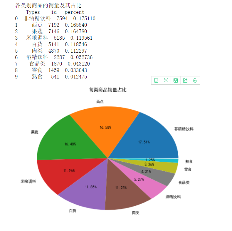
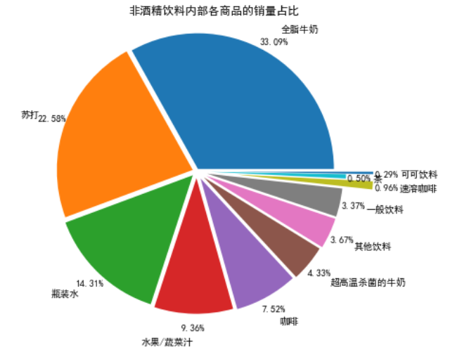
According to our analysis, the proportion of non-alcoholic beverages is the highest, accounting for 17.51%, which is the sales force. Therefore, we analyze the commodity structure of non-alcoholic beverages.
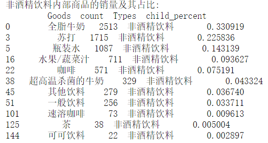
selected = sort_links.loc[sort_links['Types'] == 'Non-alcoholic Drinks']  # Select the commodity category as "non-alcoholic beverage" and sort it
child_nums = selected['id'].sum()  # Sum all "non-alcoholic beverages"
selected['child_percent'] = selected.apply(lambda line: line['id']/child_nums,axis = 1)  # Find percentage
selected.rename(columns = {'id':'count'},inplace = True)
print('Sales volume and proportion of non-alcoholic beverages:\n',selected)
# outfile2 = '../tmp/child_percent.csv'
# sort_link.to_csv(outfile2,index = False,header = True,encoding='gbk')  # Output results

# Draw a pie chart to show the proportion of sales of various commodities within non-alcoholic drinks
import matplotlib.pyplot as plt
data = selected['child_percent']
labels = selected['Goods']
plt.figure(figsize = (8,6))  # Set canvas size
explode = (0.02,0.03,0.04,0.05,0.06,0.07,0.08,0.08,0.3,0.1,0.3)  # Set the gap size of each block
plt.pie(data,explode = explode,labels = labels,autopct = '%1.2f%%',
        pctdistance = 1.1,labeldistance = 1.2)
plt.rcParams['font.sans-serif'] = 'SimHei'
plt.title("Proportion of sales volume of non-alcoholic beverages by commodity")  # Set title
plt.axis('equal')
# plt.savefig('../tmp/child_persent.png')  # Save drawing
plt.show()  # Display graphics
Here we are doing data conversion. Each line of the previous data represents each commodity and the corresponding id.
import pandas as pd
inputfile =open("C://Users / / administrator / / desktop / / Python code / / Python data analysis and mining (2nd Edition) source data and code / / Python data analysis and mining (2nd Edition) source data and code - chapters / / Chapter8 / / demo / / data / / goodorder csv")
data = pd.read_csv(inputfile)

# Merge the "Goods" column according to the id and separate the Goods with ","
data['Goods'] = data['Goods'].apply(lambda x:','+x)
print(data.head(10))

data = data.groupby('id').sum().reset_index()
print(data.head(10))

# Convert data format for merged product columns
data['Goods'] = data['Goods'].apply(lambda x :[x[1:]])#Convert to array
data_list = list(data['Goods'])

# Split the product name for each element
data_translation = []
for i in data_list:
    p = i[0].split(',')
    data_translation.append(p)
print('First 5 elements of data conversion results:\n', data_translation[0:5])
Original data:
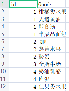
Converted data:
Convert all the goods bought by the customer with id 1 into a list. Similarly, customers with id 2 buy

5. Correlation analysis
5.1 steps of modeling implementation:
- First, set the minimum support and minimum confidence of Apriori and input the modeling sample data
- Apriori correlation analysis algorithm is used to analyze the modeling sample data, and the parameters set by the model are taken as the conditions and objectives
At present, there is no unified standard for how to set the minimum support and minimum confidence. Most of them are through setting the initial value, and then through continuous adjustment to obtain the association results consistent with the business. The model parameters input in this paper are: minimum support 0.02 and minimum confidence 0.35.
# -*- coding: utf-8 -*-

# Code 8-6 build association rule model

from numpy import *

def loadDataSet():
    return [['a', 'c', 'e'], ['b', 'd'], ['b', 'c'], ['a', 'b', 'c', 'd'], ['a', 'b'], ['b', 'c'], ['a', 'b'],
            ['a', 'b', 'c', 'e'], ['a', 'b', 'c'], ['a', 'c', 'e']]

def createC1(dataSet):
    C1 = []
    for transaction in dataSet:
        for item in transaction:
            if not [item] in C1:
                C1.append([item])
    C1.sort()
    # If the mapping is frozenset unique, you can use it to construct a dictionary
    return list(map(frozenset, C1))

# From candidate K-itemset to frequent K-itemset (support calculation)
def scanD(D, Ck, minSupport):
    ssCnt = {}
    for tid in D:   # Traversal data set
        for can in Ck:  # Traversal candidate
            if can.issubset(tid):  # Judge whether the candidate contains the items of the dataset
                if not can in ssCnt:
                    ssCnt[can] = 1  # Exclusive set to 1
                else:
                    ssCnt[can] += 1  # If yes, add 1 to the count
    numItems = float(len(D))  # Dataset size
    retList = []  # L1 initialization
    supportData = {}  # Record the support of each data in the candidate
    for key in ssCnt:
        support = ssCnt[key] / numItems  # Calculate support
        if support >= minSupport:
            retList.insert(0, key)  # Join L1 if conditions are met
            supportData[key] = support
    return retList, supportData

def calSupport(D, Ck, min_support):
    dict_sup = {}
    for i in D:
        for j in Ck:
            if j.issubset(i):
                if not j in dict_sup:
                    dict_sup[j] = 1
                else:
                    dict_sup[j] += 1
    sumCount = float(len(D))
    supportData = {}
    relist = []
    for i in dict_sup:
        temp_sup = dict_sup[i] / sumCount
        if temp_sup >= min_support:
            relist.append(i)
# Here you can set to return all the support data (or the support data of frequent itemsets)
            supportData[i] = temp_sup
    return relist, supportData

# Improved pruning algorithm
def aprioriGen(Lk, k):
    retList = []
    lenLk = len(Lk)
    for i in range(lenLk):
        for j in range(i + 1, lenLk):  # Pairwise traversal
            L1 = list(Lk[i])[:k - 2]
            L2 = list(Lk[j])[:k - 2]
            L1.sort()
            L2.sort()
            if L1 == L2:  # If the first k-1 items are equal, they can be multiplied, which can prevent duplicate items
                # Prune (a1 is an element in the k-item set, and b is a subset of all its k-1 items)
                a = Lk[i] | Lk[j]  # a is the frozenset() set
                a1 = list(a)
                b = []
                # Traversal takes out each element, converts it to set, removes the element from a1 in turn, and adds it to b
                for q in range(len(a1)):
                    t = [a1[q]]
                    tt = frozenset(set(a1) - set(t))
                    b.append(tt)
                t = 0
                for w in b:
                    # When b (that is, all subsets of k-1 items) are subsets of Lk (frequent), it is retained, otherwise it is deleted.
                    if w in Lk:
                        t += 1
                if t == len(b):
                    retList.append(b[0] | b[1])
    return retList

def apriori(dataSet, minSupport=0.2):
# The first three statements are to calculate and find the frequent itemsets in a single element
    C1 = createC1(dataSet)
    D = list(map(set, dataSet))  # Convert to a list using list()
    L1, supportData = calSupport(D, C1, minSupport)
    L = [L1]  # Add a list box so that 1 item set is a single element
    k = 2
    while (len(L[k - 2]) > 0):  # Are there any candidate sets
        Ck = aprioriGen(L[k - 2], k)
        Lk, supK = scanD(D, Ck, minSupport)  # scan DB to get Lk
        supportData.update(supK)  # Add the key value pair of supportk to supportData
        L.append(Lk)  # The last value of L is an empty set
        k += 1
    del L[-1]  # Delete the last empty set
    return L, supportData  # L is a frequent itemset, a list, and 1, 2, and 3 itemsets are elements respectively

# Generate all subsets of the collection
def getSubset(fromList, toList):
    for i in range(len(fromList)):
        t = [fromList[i]]
        tt = frozenset(set(fromList) - set(t))
        if not tt in toList:
            toList.append(tt)
            tt = list(tt)
            if len(tt) > 1:
                getSubset(tt, toList)

def calcConf(freqSet, H, supportData, ruleList, minConf=0.7):
    for conseq in H:  #Traverse all itemsets in H and calculate their confidence values
        conf = supportData[freqSet] / supportData[freqSet - conseq]  # Reliability calculation, combined with support data
        # Lift calculation lift = P (A & B) / P (a) * P (b)
        lift = supportData[freqSet] / (supportData[conseq] * supportData[freqSet - conseq])

        if conf >= minConf and lift > 1:
            print(freqSet - conseq, '-->', conseq, 'Degree of support', round(supportData[freqSet], 6), 'Confidence:', round(conf, 6),
                  'lift The value is:', round(lift, 6))
            ruleList.append((freqSet - conseq, conseq, conf))

# Generation rules
def gen_rule(L, supportData, minConf = 0.7):
    bigRuleList = []
    for i in range(1, len(L)):  # Calculate from binomial set
        for freqSet in L[i]:  # freqSet is the set of all k items
            # Find all non empty subsets of the three itemsets, 1 itemset, 2 itemsets, up to k-1 itemset, represented by H1, which is of list type and frozenset type,
            H1 = list(freqSet)
            all_subset = []
            getSubset(H1, all_subset)  # Generate all subsets
            calcConf(freqSet, all_subset, supportData, bigRuleList, minConf)
    return bigRuleList

if __name__ == '__main__':
    dataSet = data_translation
    L, supportData = apriori(dataSet, minSupport = 0.02)
    rule = gen_rule(L, supportData, minConf = 0.35)
The results are as follows:
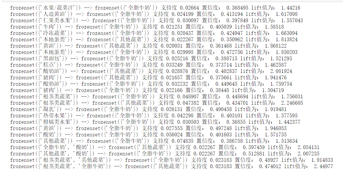
Let's explain the output results: take the first one:

This shows that the probability of buying both (fruit juice / vegetable juice) and (whole milk) is 36.85%, and the probability of this situation is 2.66%
The subsequent results can be interpreted in the same way
According to the results of the model, we find that most shoppers mainly buy food. With the improvement of living standards and the increase of health awareness, other vegetables, rhizome vegetables and whole milk are the daily food needs of modern families. Therefore, the probability of buying other vegetables, rhizome vegetables and whole milk at the same time is high, which is in line with people's life and health awareness.
6. Model application
The results of the above model show that when customers buy other goods, they will buy whole milk at the same time. Therefore, the mall should put the whole milk on the only way or in a conspicuous place for customers to take according to the actual situation. At the same time, customers are more likely to buy other vegetables, root vegetables, yogurt, pork, butter, local eggs and a variety of fruits. Therefore, shopping malls can consider bundling sales, or adjust the layout of goods to bring these goods as close as possible, so as to improve customers' shopping experience.
reference material
Link: Apriori algorithm for machine learning association rule analysis.
Book: python data analysis and mining practice
Experimental dish dataset: Data Baidu online disk download, extraction code 7hwd.