Learning objectives:
- Understand the basic principles of text mining.
- Master the method of text classification using LSTM.
Learning content:
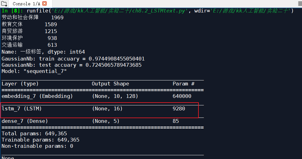
In recent years, with wechat, microblog, mayor's mailbox, sunshine hotline and other online political platforms gradually becoming an important channel for the government to understand public opinion, gather people's wisdom and condense people's morale, the amount of text data related to various social conditions and public opinion has been increasing, which has brought great challenges to the work of relevant departments that used to rely mainly on manual message division. When dealing with the mass messages on the network political platform, the staff first classify the messages according to a certain classification system, so as to assign the mass messages to the corresponding functional departments for processing. At present, most e-government systems still rely on manual processing according to experience, which has the problems of large workload, low efficiency and high error rate. Please refer to attachment text_ data. The data given by xlsx is divided into training samples and test samples. Referring to the following code, a neural network based on LSTM is established to classify the primary tags of message content. The network parameters are adjusted to improve the classification effect, and the results are compared with the original Bayesian classification method.
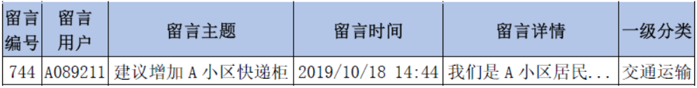
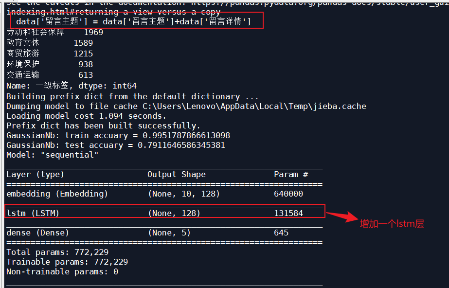
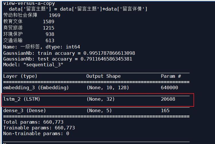
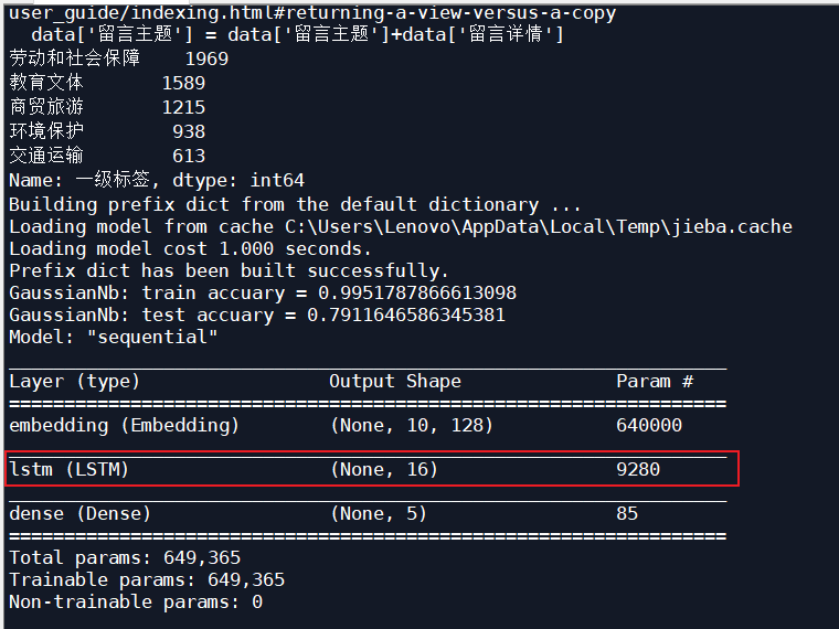
Structure of data table
Learning process:
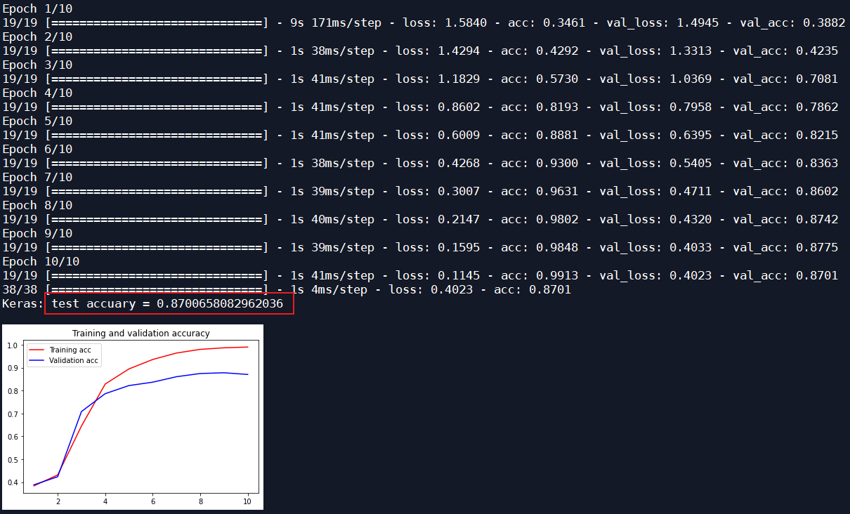
The test results are as follows:
The message subject and message details are not classified as message subject. The results of classifying the primary label of message content are shown in the table below:
| optimizer | Number of iterations | Input of LSTM_ size | Test set recognition rate | Test set recognition rate of original Bayesian classification |
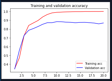
| Adam | 10 | 16 | 0.8701 | 0.7245 |
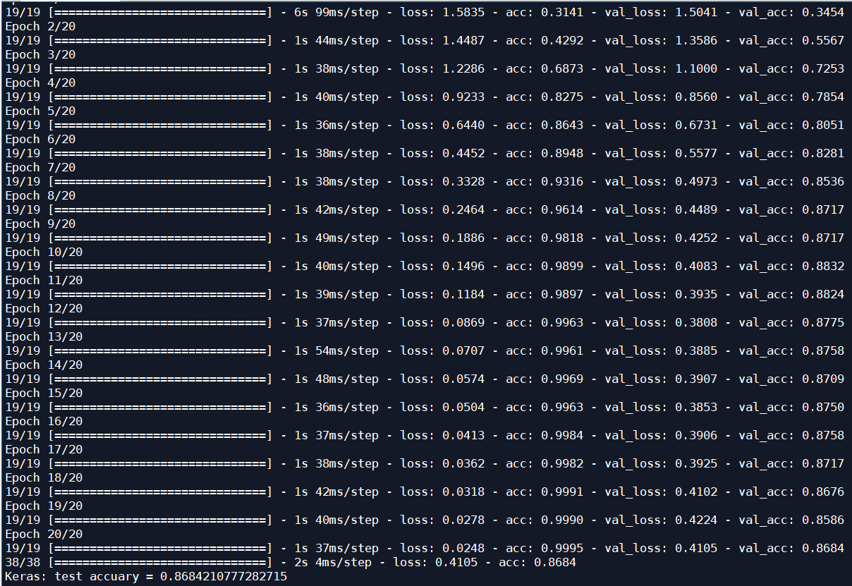
| Adam | 20 | 16 | 0.8684 | 0.7245 |
| RMSProp | 10 | 16 | 0.8692 | 0.7245 |
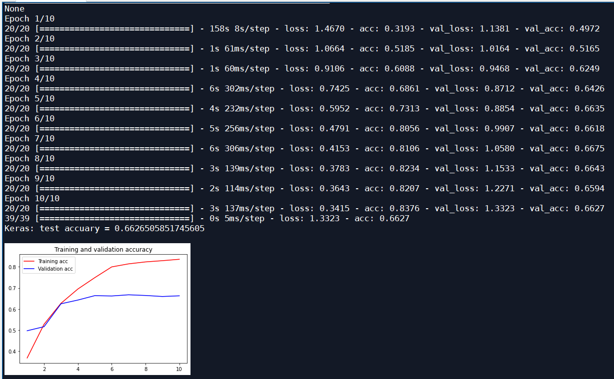
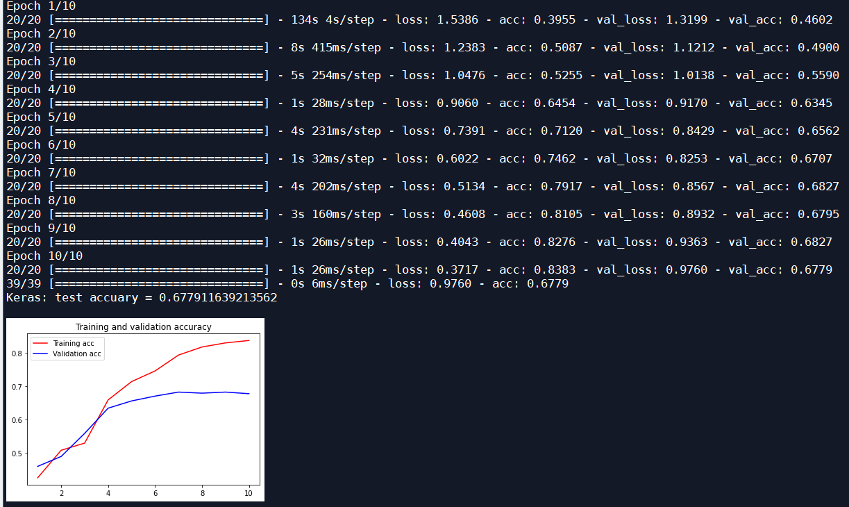
The message subject and message details are classified into the message subject. As a data set, the results of classifying the primary label of the message content are shown in the table below:
| optimizer | Number of iterations | Input of LSTM_ size | Recognition rate of test set | Test set recognition rate of original Bayesian classification |
| Adam | 10 | LSTM network not added | 0.7020 | 0.7912 |
| Adam | 10 | 128 | 0.6627 | 0.7912 |
| Adam | 10 | 32 | 0.6779 | 0.7912 |
| Adam | 10 | 16 | 0.6827 | 0.7912 |
Test process:
The message subject and message details are not classified as the message subject. The first level label of the message content is classified, an LSTM layer is added, 10 iterations, and the optimizer is Adam, input_size 16:
20 iterations:
Add an LSTM layer and iterate 10 times. The optimizer is RMSProp:
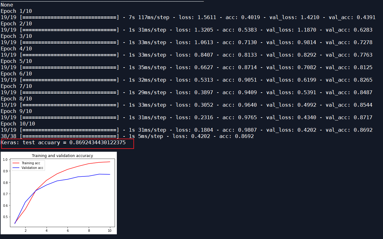
The message subject and message details are classified into the message subject, which is used as the data set to classify the primary label of the message content, and the LSTM network is not added:
Add an LSTM layer, iterate 10 times, and the optimizer is Adam input_size 128:
Add an LSTM layer, iterate 10 times, and the optimizer is Adam, input_size 32:
Add an LSTM layer, iterate 10 times, and the optimizer is Adam, input_size 16:
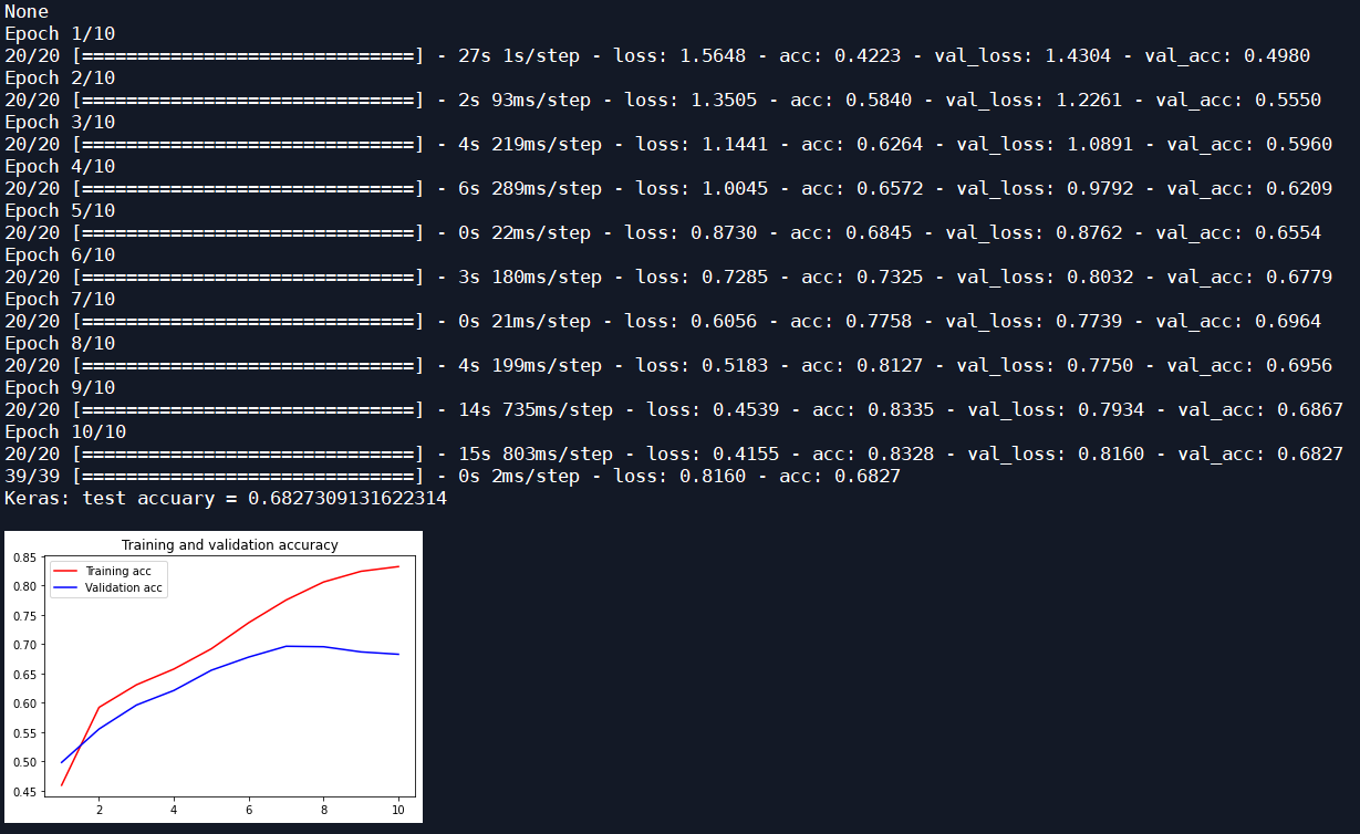
Adjust LSTM input_size, with input_ With the decrease of size, the recognition rate of test set increases gradually.
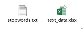
Source code:
# In[1]: reading original data
import pandas as pd
file='text_data.xlsx'
data_org = pd.read_excel(file)
data = data_org[['Message subject','Message details','Primary label']]
data['Message subject'] = data['Message subject']+data['Message details']
label_counts = data['Primary label'].value_counts()
print(label_counts)
num_class = len(label_counts)

# In[2]: Data Preprocessing
# duplicate removal
data = data['Message subject'].drop_duplicates()

# Remove x sequence
import re
data = data.apply(lambda x: re.sub('x', '', x))

# Stutter participle
import jieba
data = data.apply(lambda x:jieba.lcut(x))

# Remove stop words
stopwords=pd.read_csv('stopwords-1.txt',encoding='utf-8',sep='hhhaha',header=None,engine='python')
stopWords=['?','!','\xa0','\n','\t']+list(stopwords.iloc[:,0])
data = data.apply(lambda x:[i for i in x if i not in stopWords])

# Get label
labels = data_org.loc[data.index,'Primary label']
labels = labels.factorize()[0] # Category digitization

# Divide training samples and test samples
from sklearn.model_selection import train_test_split
data_tr,data_te,labels_tr,labels_te=train_test_split(data,labels,test_size=0.2,random_state=123)

# In[3]: use the word frequency statistics tool in the sklearn module to digitize
from sklearn.feature_extraction.text import CountVectorizer, TfidfTransformer

# The list can only be used as a countvectorizer if it is converted to a string fit_ Parameters of transform
data_tr_s=data_tr.apply(lambda x:' '.join(x))
data_te_s=data_te.apply(lambda x:' '.join(x))

 # For the word frequency of each word, all samples have the same number of columns (= the number of all words), and each column corresponds to the number of occurrences of a word
 # Some columns may have elements larger than 1, most of which are 0
countVectorizer=CountVectorizer()
data_tr_sn=countVectorizer.fit_transform(data_tr_s)

# So that all the components of each sample add up to 1
X_tr=TfidfTransformer().fit_transform(data_tr_sn.toarray()).toarray()

# Transform test sample
data_te_sn = CountVectorizer(vocabulary=countVectorizer.vocabulary_).fit_transform(data_te_s)
X_te = TfidfTransformer().fit_transform(data_te_sn.toarray()).toarray()

# In[4]: classification using Bayesian classifier
from sklearn.naive_bayes import GaussianNB
model=GaussianNB()
model.fit(X_tr,labels_tr)
score_tr = model.score(X_tr,labels_tr)
score_te = model.score(X_te, labels_te)
print('GaussianNb: train accuary = %s' % score_tr)
print('GaussianNb: test accuary = %s' % score_te)

# In[5]: use Tokenizer in keras to number words
from tensorflow.keras.preprocessing import sequence
from tensorflow.keras.preprocessing.text import Tokenizer
num_words = 5000
tokenizer = Tokenizer(num_words = num_words) #Consider only the most commonly used first num_words words
tokenizer.fit_on_texts(data_tr)
K_tr = tokenizer.texts_to_sequences(data_tr)
K_te = tokenizer.texts_to_sequences(data_te)

# Each sample has maxlen words, otherwise fill in 0 or intercept
maxlen = 10
K_tr = sequence.pad_sequences(K_tr, maxlen=maxlen)
K_te = sequence.pad_sequences(K_te, maxlen=maxlen)

# In[6]: building neural network model
from tensorflow.keras.models import Sequential
from tensorflow.keras.layers import Dense
#from keras.layers import Flatten
from tensorflow.keras.layers import LSTM
from tensorflow.python.keras.layers.embeddings import Embedding
model = Sequential()
# Embedding class converts positive integers (indexes) into dense vectors of fixed size, and reduces the dimension of data through matrix multiplication.
emebdding_layer = Embedding(num_words, 128, input_length=maxlen)
model.add(emebdding_layer)
#model.add(LSTM(128,return_sequences=True)) #Can be changed to other parameters
model.add(LSTM(16)) #Resizable
#model.add(Flatten())
model.add(Dense(num_class, activation='sigmoid')) #softsign
model.compile(optimizer='adam', loss='sparse_categorical_crossentropy', metrics=['acc']) #It can be changed to other optimizers, rmsprop,adam
print(model.summary())

# Training network
history = model.fit(K_tr,labels_tr,
                    validation_data=(K_te, labels_te),
                    batch_size=256, epochs=20)

loss, score_te = model.evaluate(K_te, labels_te)
print('Keras: test accuary = %s' % score_te)

# In[7]: draw the change of recognition rate and loss during training
import matplotlib.pyplot as plt
acc = history.history['acc']
val_acc = history.history['val_acc']
loss = history.history['loss']
val_loss = history.history['val_loss']
epochs = range(1, len(acc) + 1)

plt.title('Training and validation accuracy')
plt.plot(epochs, acc, 'red', label='Training acc')
plt.plot(epochs, val_acc, 'blue', label='Validation acc')
plt.legend()
plt.show()
Learning output:
- After adding an LSTM neural network, the recognition rate of the test set decreased. I adjusted the input of LSTM_ Size increases the recognition rate of test set;